I think the first time I really heard much about the Earth's crust was on the TV show "Bill Nye the Science Guy." (In fact, I was obsessive about not missing an episode as a child and I was ecstatic when I got to see Bill speak at Penn State last year.) He talked about earthquakes and Earth's structure, cut in with funny segments of a family telling their son, "Ritchie, eat your crust."
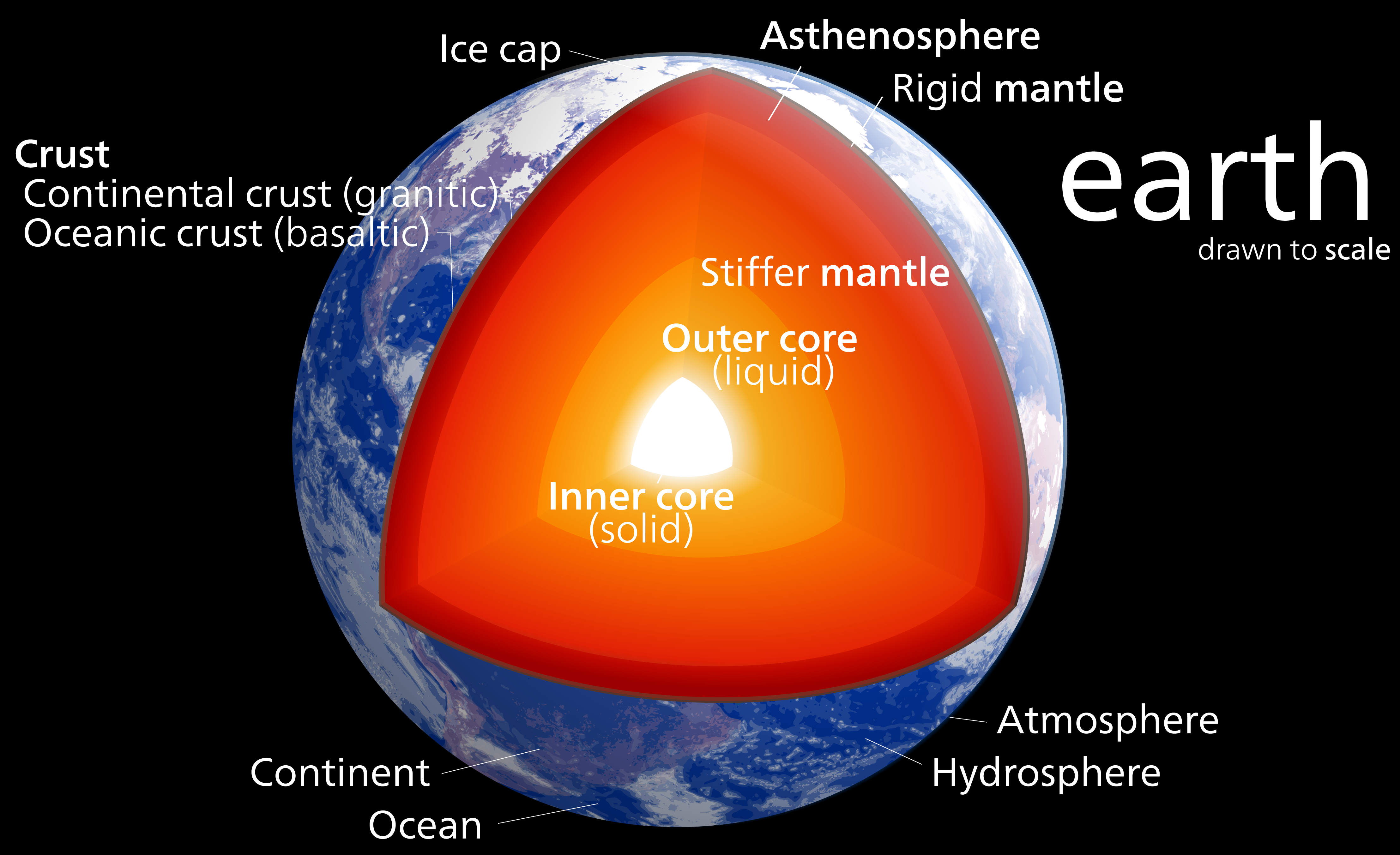
The crust in an interesting thing - it's what we live on top of and there are lots of interesting places where it's different due to geologic processes that concentrate certain types of materials. The crust is broken up into around a dozen major tectonic plates that move at about 4-6"/year. These plates are either oceanic or continental crust. Oceanic crust is generally relatively thin ~6 km (4 miles) and oceanic crust is much thicker at ~35 km (22 miles). The thin oceanic crust is also more mafic and dense than the felsic continental crust.
These differences create complex interactions when the plates meet each other at plate boundaries. We did a whole show on plate tectonics over at the Don't Panic Geocast recently, so if you'd like to hear about the discovery and arguments over plate tectonics you should check it out.
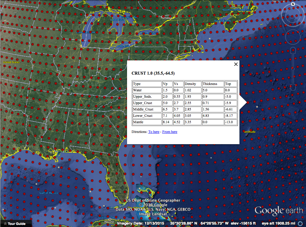
Today, I'd like to share a tool and Dr. Charles Ammon and I have made to visualize a crust model and allow anyone to explore the crust. All you need is Google Earth! We used a model called Crust 1.0 by Laske et al. that has how thick the crust (broken up into a few divisions) is for 64,800 points on the Earth along with some other crustal properties. That's every one degree of latitude and longitude! They put a lot of work into making this model. Generally we would use a Fortran program to get values out of the model, but Dr. Ammon had an idea to visualize the data in a more intuitive way with Google Earth. Over the Thanksgiving holiday I wrote a Python utility to access the model values and then we wrote a simple script that generates a Google Earth KML file based on the model.
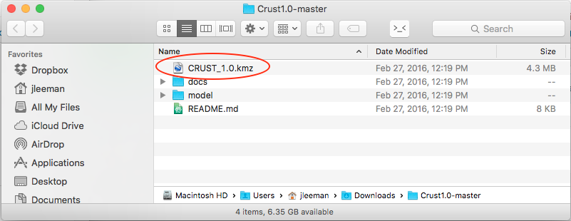
All you have to do is head over to the project's GitHub page and click the "Download ZIP" button. While you're waiting on the download you can scroll down and read all about the development, the model, and find activities to try. Next, open folder you downloaded (most operating systems will automatically unzip it for you now) there will be several files, but the only one you need is the CRUST_1.0.kmz file.
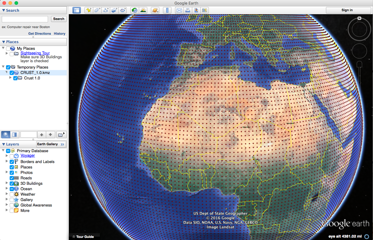
As long as you have Google Earth installed, double click that file and you'll see the Earth appear covered in red dots. If you zoom out too far, they will disappear though!
Each red dot is a location where the model has the average crustal properties like how fast P and S seismic waves can travel and the density. All of these are explained in more detail on the project webpage. You should also try some of the projects we have listed there! As a starter, let's look at oceanic and continental crust and verify my assertion about their 3x thickness difference.
Clicking out in the Atlantic Ocean (make sure you are not on the continental shelf) we see about 13 km thick crust (the top of the mantle number). The water depth is also handy to have on-hand sometimes.
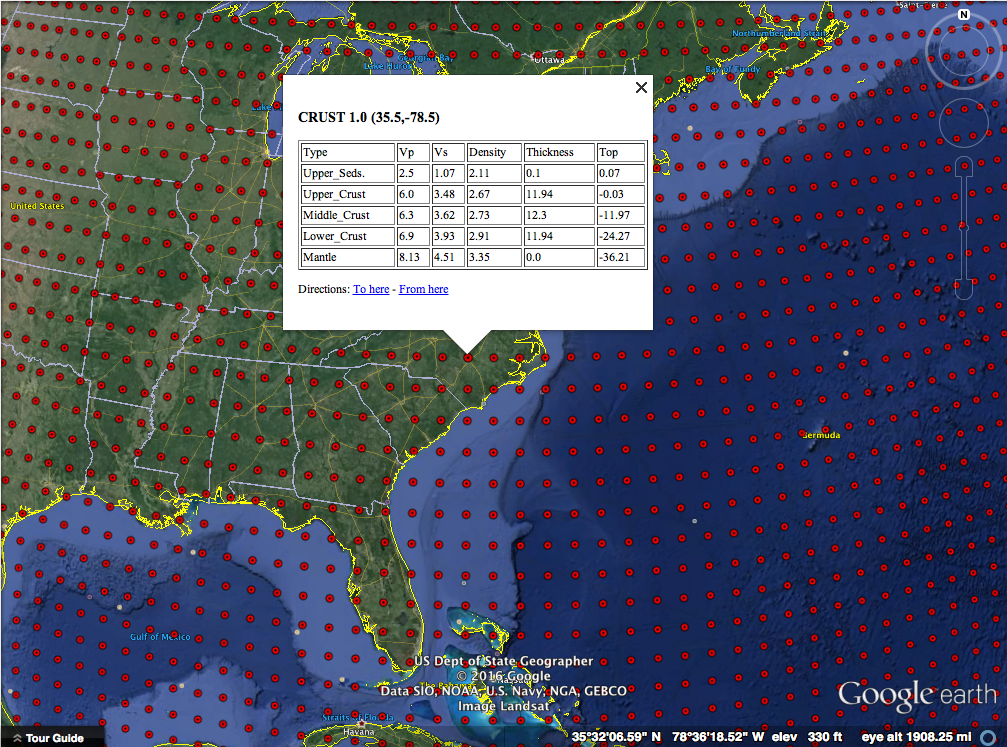
Clicking well onto the North American plate we see about 36 km thick crust. Next you should head over to mountainous regions and basins and see how the structure of the crust is different - why is that? Sorry, no homework answers here!
This is a really fun way to learn about the crust and a good reference tool as well! There are flyers in the docs folder that you can print to use as teaching aids or handout to students! We had a lot of fun making this 1-day project and hope that you'll explore it and let us know what you think! A big thanks to the folks that did the massive amount of work making the model - we just made it visible in Google Earth! Everything is open-source as always.
I've been working on developing some geophysical instruments that will need some significant temperature compensation. Often times when you buy a sensor there is some temperature dependance (if not humidity, pressure, and a slew of other variables). The manufacturer will generally quote a compensation figure. Say we are measuring voltage with an analog-to-digital converter (ADC); the temperature dependance may be quoted as some number of volts per degree of temperature change over a certain range of voltages and temperatures. Generally this is a linear correction. Most of the time that is good enough, but for scientific applications we sometimes need to squeeze out every error we can and compare instruments. Maybe one sensor is sightly more temperature dependent than another; comparing the sensors could then lead us to some false conclusions. This means that sometimes we need to calibrate every sensor we are going to use. In the lab I work in, we calibrate all of our transducers every 6 months by using transfer standards. (Standards, transfer of standards, and calibration theory are a whole series of posts in themselves.)
To do thermal calibrations it is common to put the instruments into a thermal chamber in which we can vary the temperature over a wide range of conditions while keeping the physical variable we are measuring (voltage, pressure, load, etc) constant. Then we know any change in the reading is due to thermal effects on the system. If we are measuring something like tilt or displacement, we have to be sure that we are calibrating the electronics, not signals from thermal expansion of metals and materials that make up our testing jig.
I scoured EBay and the surplus store at our University, but only found very large and expensive units. I remembered that several years ago Dave Jones over at the EEVBlog had mentioned a cheap alternative made from a peltier device wine cooler. I dug up his video (below) and went to the web again in search of the device.
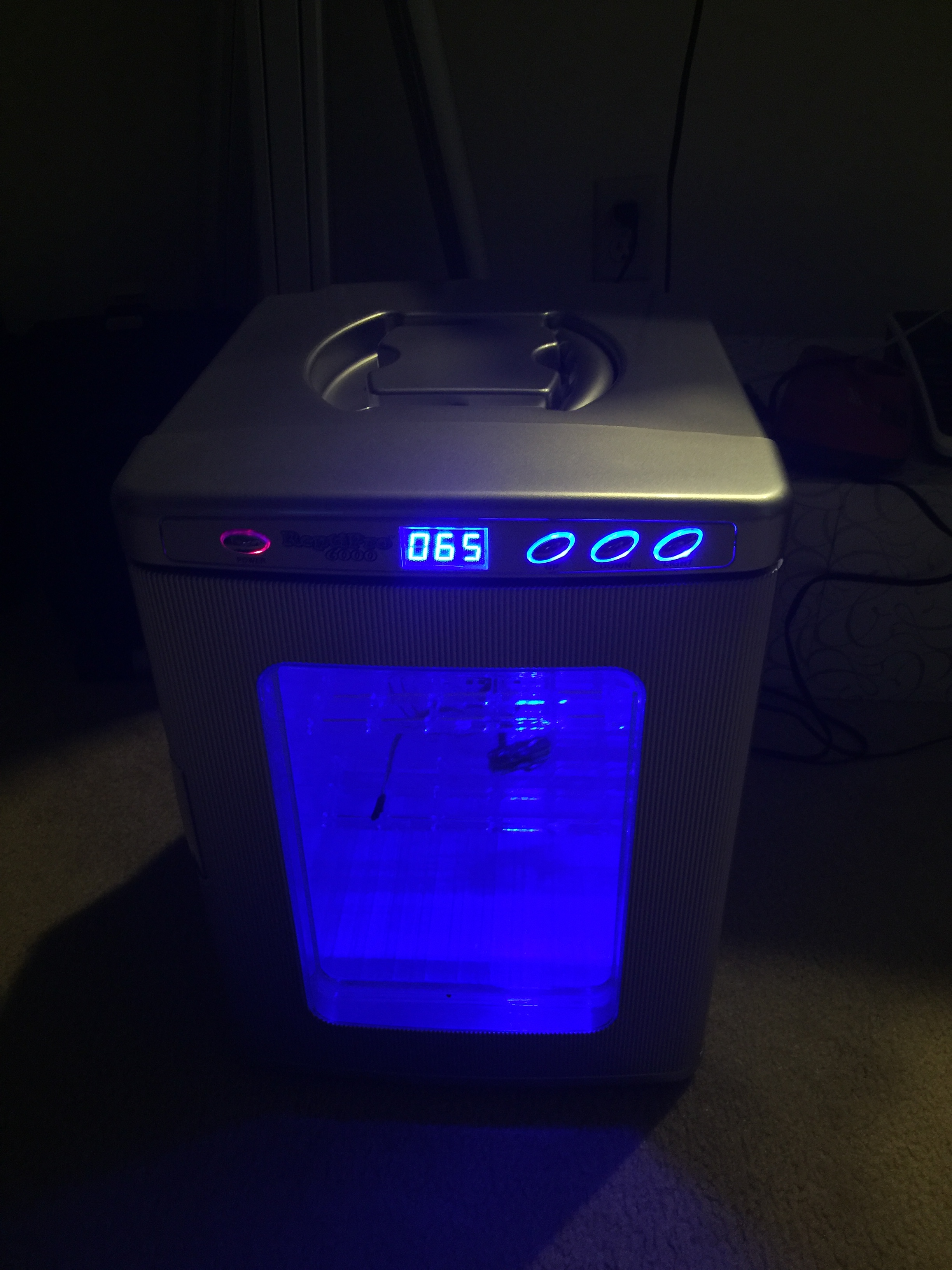
I found the chamber marketed as a reptile egg incubator on Amazon. The reviews were not great, some saying the unit was off by several degrees or did not maintain the +/- 1 degree temperature as marketed. I decided to give it a shot since it was the only affordable alternative and if it didn't work, maybe I could hack it with a new control system and use the box/peltier element with my own system. In this post I'm going to show you the stock performance of the chamber and some initial tests to figure out if it will do the job.
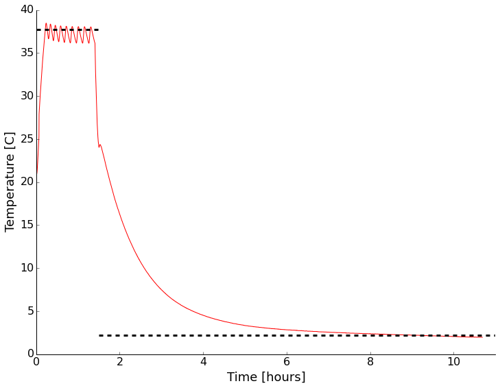
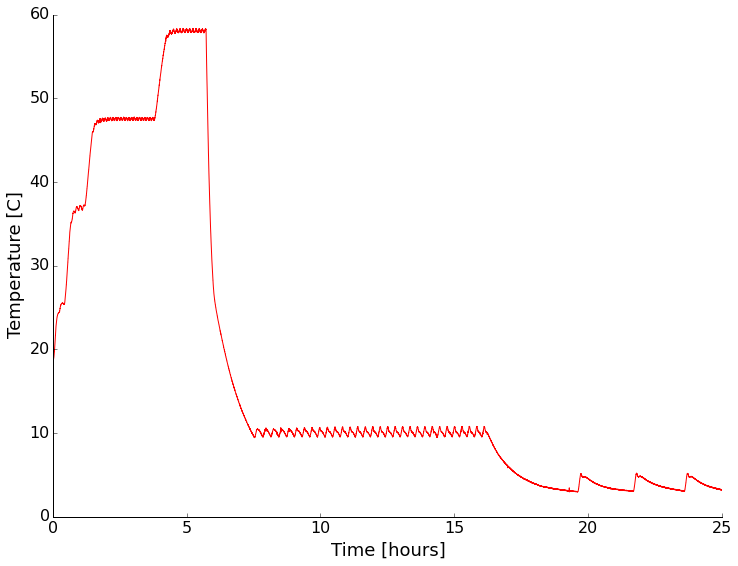
As soon as it arrived I setup the unit and put an environmental sensor in (my WxBackpack for the Light Blue Bean used back in the drone post) inside. I wanted to see if it was even close to the temperature displayed on the front and how good the control was with no thermal load inside. There was a small data drop-out causing a kink early in the record (around 30 C). It looks like the temperature is right on what I had set it to with the quoted +/- 1 degree range. There is some stabilization time and the mean isn't the same as the set point, but that makes sense to me, you don't want to overheat eggs! This looks encouraging overall. I also noticed that the LED light inside the chamber flickered wildly when the peltier device was drawing a lot of power heating/cooling the system. I then opened the door and set the unit to cool. After reaching room temperature, I closed the door and went to bed. It certainly isn't fast, but I was able to get down to about 2C with no thermal load. That was good enough for me. Time to add a cable port, checkout the LED issue, and test with some water jars for more thermal mass.
Initial test of the thermal chamber with nothing inside except a temperature logger. Set point shown by dashed line.
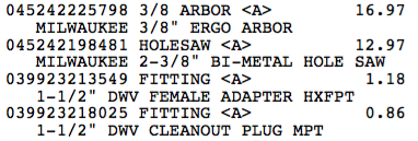
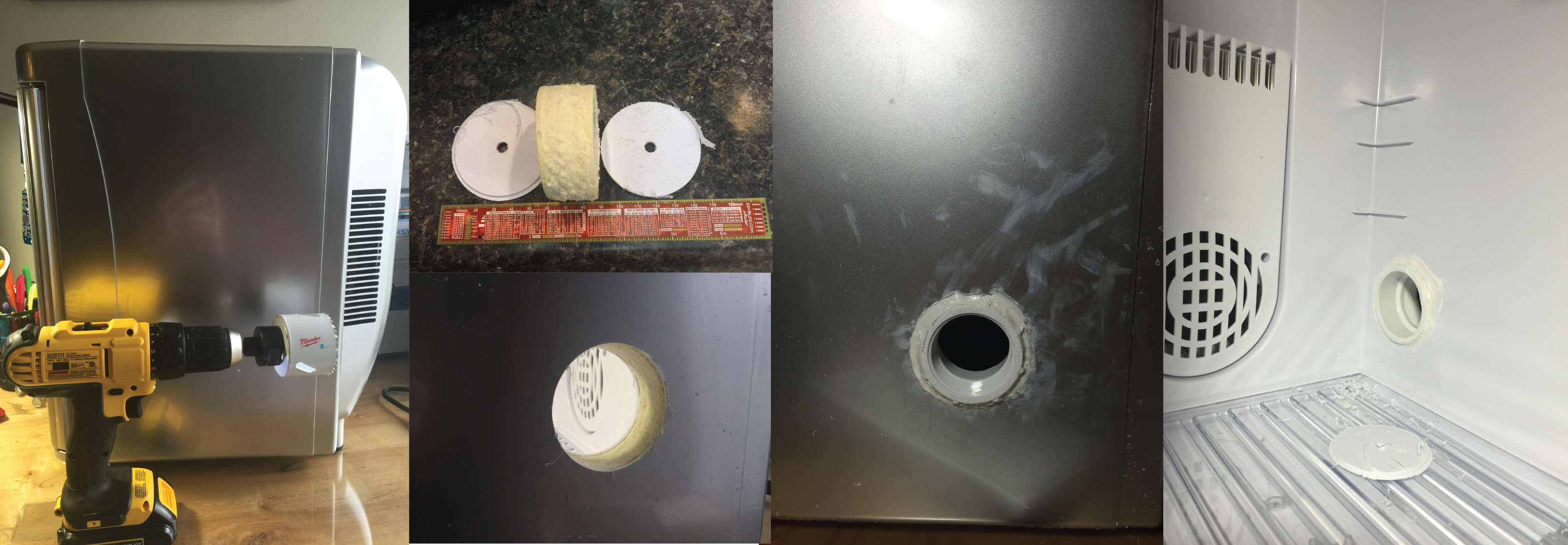
The next step was to add a cable port to be able to get test cables in and out. I decided to follow what Dave did and add a 1.5" test port with a PVC fitting, a hole saw, and some silicone sealant. Below are a few pictures of drilling and inserting the fitting. I used Home Depot parts (listing below). I didn't have the correct size hole-saw. That's happened a lot lately, so I invested in the Milwaukee interchangeable system. I got a threaded fitting so I can put a plug in if needed. the time honored tradition is to put your cables through the port and stuff a rag in though. This works as well as a plug generally, but it's nice to have the option.
Before, during, and after cable port placement. The center of the hole is 7 3/8" back from the front door seal, and 5 1/8" up from table top level. I used gel super glue to quickly fix the fitting to the plastic layers and foam. After that dried, I used silicone bath adhesive/sealant to seal the inside and outside. The edge of a junk-mail credit card offer made smoothing the silicone easier.
While working inside the chamber I pulled out the LED board and noticed a dodgy looking solder joint. I reflowed it. I also pulled the back off the unit to make sure there were no dangerous connections or anything that looked poor quality. Nothing jumped out.
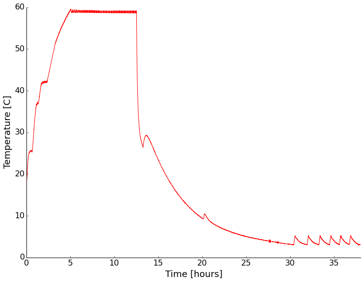
I put the whole thing back together and put a sensor in to monitor the environment and tested again. This time I tried a few different set points with and without containers of water inside the chamber. First with nothing but the sensor setup inside:
For both heating and cooling the performance under no thermal load (other than the sensor electronics) was pretty good. Cooling is rather slow and more poorly controlled than heating though.
Next I put sealed containers of water on the shelves of the chamber to add some thermal mass and see if that changed the characteristics of the chamber any. It did slow the temperature change as expected, but appears to have had little other effect (I didn't wait long enough for stabilization on some settings).
With a water load the chamber had similar performance, but was slower in getting to temperature as expected.
It looks like at temperatures above ambient the chamber has a stability of +/- 1 degree. Below ambient it becomes a couple of degrees. The absolute reading drifts a bit too. Setting the chamber to a given reading always resulted in stabilization within about a degree of the setting though.
I think this will be a nice addition to my home lab. While the unit isn't incredibly accurate, I will be recording the device temperature anyway, so that works for me. It'd be nice to cool down more quickly though, so I may facilitate that with some dry ice. Stay tuned as I'll be testing instruments in there sometime in the next month or so.
P.S. - The LED light still flickers in a way that indicates unstable power/connection. Not a deal breaker for me since I don't really need the light, but something to remember.
I end up doing a lot of debugging, in fact every single day I'm debugging something. Some days it is software and scripts that I'm using for my PhD research, some days it is failed laboratory equipment, and some days it's working the problems out of a new instrument design. Growing up working on mechanical things really helped me develop a knack for isolating problems, but this is not knowledge that everyone has the occasion to develop. I'm always looking for ways to help people learn good debugging techniques. There's nothing like discovering, tracking down, and fixing a bug in something. Also, the more good debuggers there are in the world, the fewer hours are waisted fruitlessly guessing at problems.
I'd heard about a debugging book that was supposed to be good for any level of debugger, from engineer to manager to homeowner. I was a little suspicious since the is such a wide audience, but I found that my library had the book and checked it out; it is "Debugging: The 9 Indispensable Rules for Finding Even the Most Elusive Software and Hardware Problems" by David Agans. The book sat on my shelf for a few months while I was "too busy" to read it. Finally, I decided to tackle a chapter a day. The chapters are short and I can handle two weeks of following the book. Each morning when I got to work, I read the chapter for that day. One weekend I read an extra chapter or two because they were enjoyable.
I'm not going to ruin the book, but I am going to tell you the 9 rules (it's okay, they are also available in poster form on the book website).
Understand the System
Make It Fail
Quit Thinking and Look
Divide and Conquer
Change One Thing at a Time
Keep an Audit Trail
Check the Plug
Get a Fresh View
If You Didn't Fix It, It Ain't Fixed
They seem simple, but think of the times you've tried to fix something and skipped around because you thought you knew better to have it come back to sting you. If you've done a lot of debugging, you can already see the value of this book.
The book contains a lot of "war stories" that tell tales of when a rule or several rules were the key in a debugging problem. My personal favorite was the story about a video conferencing system that seemed to randomly crash. Turns out the compression of the video had problems with certain patterns and when the author wore a plaid shirt to work and would test the system, it failed. He ended up sending photocopies of his shirt to the manufacturer of the chip. Fun stories like that made the book fun to read and show how you have to pay attention to everything when debugging.
The book has a slight hardware leaning, but has examples of software, hardware, and home appliances. I think that all experimentalists or engineers should read this early on in their education. It'll save hours of time and make you seem like a bug whisperer. Managers can learn from this too and see the need to provide proper time, tools, and support to engineering.
If you like the blog, you'll probably like this book or know someone that needs it for Christmas. I am not being paid to write this, I don't know the author or publisher, but wanted to share this find with the blog audience. Enjoy and leave any comments about resources or your own debugging issues!
Last time I wrote up the basics of a tip sent in by Evan over at Agile Geoscience. This technology is very neat, if you haven't read that post first, please do and watch the TED talk. This post is going to be about how we could apply this to problems in geoscience. Some of these ideas are "low hanging fruit" that could be relatively easy to accomplish, others are in need of a few more PhD students to flesh them out. I'd love to work on it myself, but I keep hearing about this thing called graduation and think it sounds like a grand time. Maybe after graduation I can play with some of these in detail, maybe before I can just experiment around a bit.
In his email to me, Evan pointed out that this visual microphone work IS seismology of sorts. In seismology we look at the motion of the Earth with seismometers or geophones. If we have a lot of them and can look at the motion of the Earth in a lot of places over time, we can learn a lot about what it's like inside the Earth. This type of survey has been used to understand problems as big as the structure of the Earth and as small as finding artifacts or oil in shallow deposits. In (very) general terms we look at very low frequency waves for Earth structure problems with periods of a second to a few hundred seconds. For more near surface problems we may look at signals up to a few hundred cycles per second (Hz). Remember in the last post I said that we collect audio data at around 44,200 Hz? That's because as humans we are able to hear up to around 20,000 Hz. All of this is a lot higher frequency than we ever use in geoscience... I'm thinking that makes this technique somewhat easier to apply and maybe even able to use poor quality images.
So what could it be used for? Below are a few bullet points of ideas. Please add to them in the comments or tear them apart. I agree with Evan that there is some great potential here.
Find/visualize/simulate stress and strain concentration in heterogeneous materials.
Extract modulus of rock from video of compression tests. Could be as simple as stepping on the rock.
Extend the model to add predicted failure and show expected strain right before failure.
Look at a sample from multiple camera views and combine for the full anisotropic properties. This smells of some modification of structure from motion techniques.
Characterize complicated machines stiffness/strain to correct for it when reducing experimental data without complex models for the machine.
Try prediction of building response during shaking.
What about perturbing bodies of water and modeling the wave-field?
With everything in science, engineering, and life, there are tradeoffs. What are the catches here? Well, the resolution is pretty good, but may not be good enough for the small differences in properties we sometimes deal with. In translating this over to work on seismic data I think a lot of algorithm changes would have to happen that may end up making it about the same utility as our first-principles approaches. A big limitation for earthquake science is what happens at large strains. The model looks at small strains/vibrations to model linear elastic behavior. That's like stretching a spring and letting it spring back (remember Hooke's Law?). Things get interesting in the non-linear part of deformation when we permanently deform things. Imagine that you stretch the spring above much further than it was designed to be. The nice linear-elastic behavior would go away and plastic deformation would start. You'd deform the spring and it wouldn't ever spring back the same way it was again. Eventually, as you keep stretching, the spring would break. The non-linear parts of deformation are really important to us in earthquake science for obvious reasons. For active seismic survey people, the small strain approximation isn't bad though.
Another issue I can imagine is combining video from different orientations to recover the full behavior of the material. I don't know all of the details of Abe's algorithm, but I think it would have problems with anisotropic materials. Those are materials that behave differently in different directions. Imagine a cube that can be easily squeezed on two opposing faces, but not easily squeezed on the others. Some rocks behave in such a way (layered rocks in particular). That's really important since they are also common rocks for hydrocarbon operations to target! Surrounding the sample area with different views (video or seismic) and using all of that information should do the job, but it's bound to be pretty tricky.
The last thing that strikes me is processing time. I don't think I've seen any quotes of how long the processing of the video clips took to recover the audio. While I don't think it's ludicrous, I think the short clips could conceivably take a few hours per every 10 seconds (this is a guess). For large or long duration geo experiments that could become an issue.
So what's the end story? Well, I think this is a technology that we haven't seen the last of. The techniques are only going to get better and processors faster to let us do more number crunching. I'm curious to watch this develop and try to apply it in some basic experiments and see what happens. What would you try this technique on? Leave it in the comments!
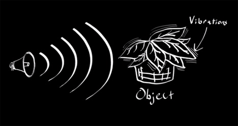
Today I wanted to share some thoughts on some great new technology that is being actively developed and uses cameras to extract sound and physical property information from everyday objects. I had heard of the visual microphone work that Abe Davis and his cohorts at MIT were working with, but they've gone a step further recently. Before we jump in, I wanted to thank Evan Bianco of Agile Geoscience for pointing me in this direction and asking about what implications this could have for rock mechanics. If you like the things I post, be sure to checkout Agile's blog!
Abe's initial work on the "visual microphone" consisted of using high speed cameras and trying to recover sound in a room by videoing an object like a plant or bag of chips and analyzing the tiny movements of the object. Remember sound is a propagating pressure wave and makes things vibrate, just not necessarily that much. I remember thinking "wow, that's really neat, but I don't have a high speed camera and can't afford one". Then Abe figured out a way to do this with normal cameras by utilizing the fact that most digital cameras have a rolling shutter.
Most video cameras around shoot video at 24 or 32 frames (still photos) each second (frames per second or fps). Modern motion pictures are produced at 24 fps. If we change the photos very slowly and we just see flashing pictures, but around the 16 fps mark our mind begins to merge the images into a movie. This is an effect of persistence of vision and it's a fascinating rabbit hole to crawl down. (For example, did you know that old time film projectors flashed the same frame more than once? The rapid flashing helped us not see flickers, but still let the film run at a slower speed. Checkout the engineer guy's video about this.) In the old days of film, the images were exposed all at once. Every point of light in the scene simultaneously flooded through the camera and exposed the film. That's not how digital cameras work at all. Most digital cameras use a rolling shutter. This means the image acquisition system scans across the CCD sensor row by row (much like your TV scans to show an image, called raster scanning) and records the light hitting that sensor. This means for things moving really fast, we get some strange recordings! The camera isn't designed to capture things that move significantly in a single frame. This is a type of non-traditional signal aliasing. Regular aliasing is why wagon wheels in westerns sometimes look like they are spinning backwards. Have a look at the short clip below that shows an aircraft propeller spinning. If that's real I want off the plane!
But how does a rolling shutter help here? Well 24 fps just isn't fast enough to recover audio. A lot of audio recordings sample the air pressure at the microphone about 44,200 times per second. Abe uses the fact that the scanning of the sensor gives him more temporal resolution than that rate at which entire frames are being captured. The details of the algorithm can get complex, but the idea is to watch an object vibrate and by measuring the vibration estimate the sound pressure and back-out the sound.
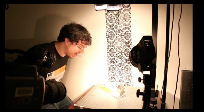
Sure we've all seen spies reflect a laser off glass in a building to listen to conversations in the room, but this is using objects in the room and simple video! Early days of the technology required ideal lighting and loud sounds. Here's Abe screaming the words to "Mary had a little lamb" at a bag of potato chips for a test.... not exactly the world of James Bond.
As the team improved the algorithm, they filmed the bag in a natural setting through a glass pane and recovered music. Finally they were able to recover music from a pair of earbuds laying on a table. The audio quality isn't perfect, but good enough that Shazam recognized the song!
The tricks that the group has been up to lately though are what is the most fascinating. By videoing objects that are being minority perturbed by external forces, they are able to model the object's physical properties and predict its behavior. Be sure to watch the TED talk below to see it in action. If you're short on time skip into about the 12 minute mark, but really just watch it all.
By extracting the modulus/stiffness of objects and how they respond to forces, the models they create are pretty lifelike simulations of what would happen if you exerted a force on the real thing. The movements don't have to be big. Just tapping the table with a wire figure on it or videoing trees in a gentle breeze is all it needs. This technology could let us create stunning effects in movies and maybe even be implemented in the lab.
I've got some ideas on some low hanging fruit that could be tried and some more advanced ideas as well. I'm going to talk about that next time (sorry Evan)! I want to make sure we all have time to watch the TED video and that I can expand my list a little more. I'm thinking along the lines of laboratory sensing technology and civil engineering modeling on the cheap... What ideas do you have? Expect another post in the very near future!
For the second installment in our summer open science series, I’d like to talk about open data. This could very well be one of the more debated topics; I certainly know it always gets my colleagues opinions exposed very quickly in one direction or the other. I’d like to think about why we would do this, methods and challenges of open data, and close with my personal viewpoint on the topic.
What is Open Data?
Open data simply means putting data that supports your scientific arguments in a publicly available location for anyone to download, replicate your analysis, or try new kinds of analysis. This is now easier than ever for us to do with a vast array of services that offer hosting of data, code, etc. The fact that every researcher will likely have a fast internet connection makes most arguments about file size invalid, with the exception of very large (100’s of gigabytes) files. The quote below is a good starting place for our discussion:
Numerous scientists have pointed out the irony that right at the historical moment when we have the technologies to permit worldwide availability and distributed process of scientific data, broadening collaboration and accelerating the pace and depth of discovery…..we are busy locking up that data and preventing the use of correspondingly advanced technologies on knowledge.
- John Wilbanks, VP Science, Creative Commons
Why/Why-Not Open Data?
When I say that I put my data “out-there” for mass consumption, I often get strange looks from others in the field. Sometimes it is due to not being familiar with the concept, but other times it comes with the line “are you crazy?” Let’s take a look at why and why-not to set data free.
First, let’s state the facts about why open data is good. I don’t think there is much argument on these points, then we’ll go on to address more two-sided facets of the idea. It is clear that open data has the potential to increase the friendliness of a group of knowledge workers and the ability to increase our collaboration potential. Sharing our data enables us to pull from data that has been collected by others, and gain new insights from other’s analysis and comments on our data. This can reduce the reproduction of work and hopefully increase the numbers of checks done on a particular analysis. It also gives our supporters (tax payers for most of us) the best “bang for their buck.” The more places that the same data is used, the cost per bit of knowledge extracted from it is reduced. Finally, open data prevents researchers from taking their body of knowledge “to the grave” either literally or metaphorically. Too often a grad student leaves a lab group to go on in their career and all of their data, notes, results, etc that are not published go with them. Later students have to reproduce some of the work for comparison using scant clues in papers, or email the original student and ask for the data. After some rummaging, they are likely emailed a few scattered, poorly formatted spreadsheets with some random sampling of the data that is worse than no data at all. Open data means that quality data is posted and available for anyone, including future students and future versions of yourself!
Like every coin, there is another side to open data. This side is full of “challenges.” Some of these challenges even pass the polite term and are really just full-blown problems. The biggest criticism is wondering why someone would make the data that they worked very hard to collect out in the open, for free, to be utilized by anyone and for any purpose. Maybe you plan on mining the data more yourself and are afraid that someone else will do that first. Maybe the data is very costly to collect and there is great competition to have the “best set” of data. Whatever the motivation, this complaint is not going to go away. Generally my reply to these criticisms goes along the lines of data citation. Data is becoming a commodity in any field (marketing, biology, music, geology, etc). The best way to be sure that your data is properly obtained is to make it open with citation. This means that people will use your data, because they can find it, but provide proper credit. There are a number of ways to get your data assigned a digital object identifier (DOI), including services like datacite. If anything, this protects the data collector by providing a time-stamp of doing data collection of phenomena X at a certain time with a time-stamped data entry. I’m also very hopeful that future tenure committees will begin to recognize data as a useful output, not just papers. I’ve seen too many papers that were published as a “data dump.” I believe that we are technologically past that now, if we can get past "publish or perish," we can stop these publications and just let the data speak for itself.
Another common statement is “my data is too complicated/specialized to be used by anyone else, and I don’t want it getting mis-used.” I understand the sentiment behind this statement, but often hear it as “I don’t want to dedicate time to cleaning up my data, I’ll never look at it after I publish this paper anyway.” Taking the time to clean up data for it to be made publicly available is when you have a second chance to find problems, make notes about procedures and observations, and make it clear exactly what happened during your experiment (physical or computational). I cannot even count the number of times I’ve looked back at old data and found notes to myself in the comments that helped guide me through re-analysis. These notes saved hours of time and possibly a few mistakes along the way.
Data Licensing
Like everything from software to intellectual property, open-data requires a license to work. No license on data is almost worse that no data at all because the hands of whoever finds it are legally bound to do nothing with it. There is even a PLOS article about licensing scientific softwarethat is a good read and largely applies to data.
What data licensing options are available to you are largely a function of the country you work in and you should talk with your funding agency. The country or funding agency may limit the options you have. For example, any US publicly funded research must be available after a presidential mandate that data be open where possible “as a public good to advance government efficiency, improve accountability, and fuel private sector innovation, scientific discovery, and economic growth.” You can read all about it in the White House U.S. Open Data Action Plan. So, depending on your funding source you may be violating policy by hoarding your data.
There is one exception to this: Some data are export controlled, meaning that the government restricts what can be put out in the open for national security purposes. Generally this pertains to projects that have applications in areas such as nuclear weapons, missile guidance, sonar, and other defense department topics. Even in these cases, it is often that certain parts of the data may still be released (and should be), but it is possible that some bits of data or code may be confidential. Releasing these is a good way to end up in trouble with your government, so be sure to check. This generally applies to nuclear and mechanical engineering projects and some astrophysical projects.
File Formats
A large challenge to open data is the file formats we use to store our data. Often times the scientist will use an instrument to collect their data that stores information in a manufacturer specific, proprietary format. It is analyzed with proprietary software and a screen-shot of the results included in the publication. Posting that raw data from the instrument does no good since others must have the licensed and closed-source software to even open it. In many cases, the users pay many thousands of dollars a year for a software “seat” that allows them to use the software. If they stop paying, the software stops working… they never really own it. This is a technique that the instrument companies use to ensure continued revenue. I understand the strategy from a business perspective and understand that development is expensive, but this is the wrong business model for a research company. Especially considering that the software is generally difficult to use and poorly written.
Why do we still deal in proprietary formats? Often it is because that is what the software we use has, as mentioned above. Other times it is because legacy formats die hard. Research groups that have a large base of data in an outdated format are hesitant to update the format because it involves a lot of data maintenance. That kind of work is slow, boring, and unfunded. It’s no wonder nobody wants to do it! This is partially the fault of the funding structure, and unmaintained data is useless data and does not fulfill the “open” idea. I’m not sure what the best way to change this idea in the community is, but it must change. Recent competitions to “rescue” data from older publications are a promising start. Another, darker, reason is that some researches want to make their data obscure. Sure, it is posted online, so they claim it is “open”, but the format is poorly explained or there is no meta-data. This is a rare case, but in competitive fields can be found. This is data hoarding in the ugliest form under the guise of being open.
There are several open formats that are available for almost any kind of data including plain text, markdown, netCDF, HDF5, and TDMS. I was at a meeting a few years ago where someone argued that all data should be archived as Excel files because “you’ll always be able to open those.” My jaw dropped. Excel is a closed, XML based, format that you must have a closed-source program to open. Yes, Open Office can open those files, but compatibility can be sketchy. Stick to a format that can handle large files (unlike Excel), supports complex multi-dimensional data (unlike Excel), and has many tools in many languages to read/write it (unlike Excel).
The final format/data maintenance task is a physical format concern. Storage media changes with time. We have transitioned from tapes, floppy disks, CDs, and ZIP disks to solid state storage and large external hard-drives. I’m sure some folks have their data on large floppy disks, but haven’t had a computer to read them in years. That data is lost as well. Keeping formats updated is another thankless and unfunded task. Even modern hard-drives must be backed up and replaced after a finite shelf life to ensure data continuity. Until the funding agencies realize this, the best we can do is write in a small budget line-item to update our storage and maintain a safe and useful archive of our data.
Meta-Data
The last item I want to talk about in this already long article is meta-data. Meta-data, as the name implies, are data about the data. Without the meta-data, most data are useless. Data must be accompanied by the experimental description, relevant parameters (who, when, where, why, how, etc), and information about what each data item means. Often this data lives in the pages of the laboratory notebooks of experimenters or on scraps of paper or whiteboards for modelers. Scanners with optical character recognition (OCR) can help solve that problem in many cases.
The other problems with meta-data are human problems. We think we’ll remember something, or we don’t have time to collect it. Anytime that I’ve thought I didn’t have time to write good notes, I payed by spending much more time after the fact figuring out what happened. Collecting meta-data is something we can’t ever do enough of and need to train ourselves to do. Again, it is a thankless and unfunded job… but just do it. I’ve even just turned on a video or audio recorder before and dictated what I’m doing. If you are running a complex analysis procedure, flip on a screen capture program and make a video of doing it to explain it to your future self and anyone else who is interested.
Meta-data is also a tricky beast because we never know what to record. Generally, record everything you think is relevant, then record everything else. In rock mechanics we generally record stress conditions, but never think to write down things like temperature and humidity in the lab. Well, we never think to until someone proves that humidity makes a difference in the results. Now all of our old data could be mined to verify/refute that hypothesis, except we don’t have the meta-data of humidity. While recording everything is impossible, it is wise to record everything that you can within a reasonable budget and time commitment. Consistency is key. Recording all of the parameters every time is necessary to be useful!
Final Thoughts
Whew! That is a lot of content. I think each item has a lot unsaid still, but this is where my thinking currently sits on the topic. I think my view is rather clear, but I want to know how we can make it better. How can we share in fair and useful ways? Everyone is imperfect at this, but that shouldn’t stop us from striving for the best results we can achieve! Next time we’ll briefly mention an unplanned segment on open-notebooks, then get on to open-source software. Until then, keep collecting, documenting, and sharing. Please comment with your thoughts/opinions!
It is finally summer and I see lots of people playing all sorts of outdoor sports. While I have never been a big sports player, it is fun to watch. There are a lot of physics involved in most sports, so maybe that is a line of posts worth investigating. I do have a post series on open source science planned that will last most of the summer, but maybe we can keep sports in mind next year?
This post is a resurrection of a post I started a couple of years ago and never got around to finishing. In an effort to tie up loose ends, here we go! How does a frisbee fly? I wondered this when we discovered that my fiancée can throw a frisbee upside down sometimes with results that flew surprisingly far. To understand what is happening we need to look at the fundamental physics of frisbee flight, make some measurements, then try to draw some conclusions. Turns out there is a lot of research on the aerodynamics of flying discs, so I'll hit the important points and leave links to let you dig down the wiki-hole with me if you wish. To start out, check out a copy of "Spinning Flight" by Ralph Lorenz at your library.
The physics of frisbee flight
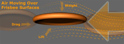
While in flight, our frisbee will experience several forces governing its movement including gravity, lift, drag, and a torque from its angular momentum. We will quickly look at each of these, but we are not going to fully model the system (though it could be fun!)
Forces on a frisbee. (Image: illumin.usc.edu)
First off, Gravity is the most obvious and intuitive of these forces. Everything is pulled towards the earth's center of mass by gravity at about 9.81m/s/s. If we just place the frisbee on the table, it will experience a force resulting from the acceleration of gravity. If we drop it, it will be accelerated downward. The velocity of falling objects has been fully investigated and we won't go into that too deeply. For now, simply assume that we could calculate the velocity of a dropped object or calculate the acceleration of an object if we know its fall rate.
Lift is what may be the most important force in this study. Believe it or not, a frisbee experiences lift following the same principles as a traditional wing or rotor blade. As the frisbee cuts through the air, some of the oncoming air goes over the frisbee, some goes under. The air streams have to meet up in the lee of the frisbee and since we cannot create or destroy air, we must have continuity and conservation. The air on top has to move faster for this to hold, it has longer to travel after all, and the air below can move more slowly. Thanks to Bernoulli's principle, we know that air moving faster will have a decreased pressure. This isn't anything new; in fact, Daniel Bernoulli published this idea in 1738! With fast air on top of the frisbee and slower air below, there is high pressure below and low pressure above the disk. From a difference in pressure we get the force of lift (more generally called a pressure gradient force).
Lift force from a pressure differential. (Image web.wellington.org)
Drag is the reason that our frisbee does not fly off into the distance. Drag is the force that slows the frisbee down as it pushes through the dense atmosphere. We could try to measure the drag through our later analysis, but that itself it a very deep task that we could spend a lot of time on.
Finally, comes the torque from the angular momentum of our frisbee. Have you tried to throw a frisbee without spinning it? In theory it would fly right? It's just a circular wing after all. Well, that turns out to be a pretty unstable way to fly your disc. Generally it will turn up, stall, and then fall like a rock. Why? Thanks to some spatial change in the lift force, the front of the disc will be lifted with slightly more force than the back, causing the disc to torque over to the back. In fact, I'll save you the trouble, you can watch my feeble attempts below. We could try to outfit our frisbee with control surfaces to help it maintain the proper angle of attack, but that is heavy, complicated, and would mean dead batteries would plague playing kids and dogs. Surely there is a more simple way?
Of course! Let's spin the frisbee when we throw it! When we throw the disc and it spins, we get gyroscopic stability and the possibility to see the cool spinning designs we print on the toy. We can determine that this torque will point vertically through the top of the frisbee. If you remember the right hand rule, you'll see that for my right-handed clockwise throw, the torque vector will point towards the ground. For the south-paws out there, your torque vector will point towards the sky. The important thing is that it will try to counteract the tendency of the lift moment to make the frisbee backflip. Granted, it will not win forever. Eventually the flight will become unstable, but we can maintain steady flight for several seconds. Depending on the force balance, we'll also expect to see the frisbee's vertical axis precess around true "up".
Taking measurements
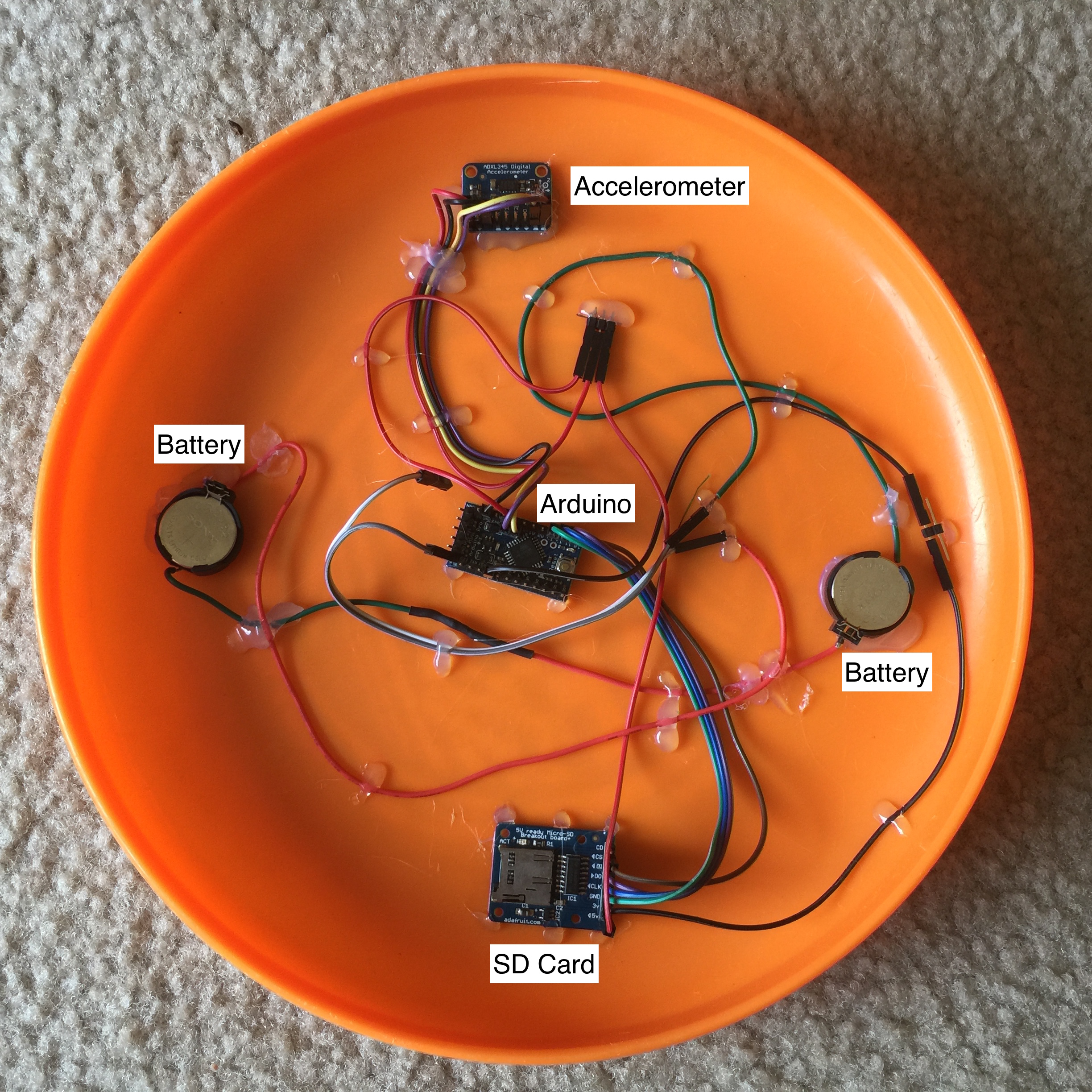
To take some measurements of frisbee flight, I created an instrumented frisbee. Turns out, I'm not the first one to do this. Lorenz made an instrumented frisbee in the early 2000's and then improved it by adding a plethorera of sensors. I decided that a simple accelerometer would be enough for my investigation. While adding angle sensors and such would be interesting, let's keep it simple for a first pass. Maybe adding a 9 degree of freedom inertial measurement unit would be fun, but that's an idea for another time. Actually, the gyroscope data from that would be incredibly useful.
I used an Arduino Pro Mini for my micro controller, an accelerometer, and SD card logger for the sensor and logging system. I ended up just trying to read the sensor in single shot mode as fast as possible. This gave a data rate of around 180-200 Hz with time-stamps in microseconds on each packet. Sure, we could make this part a little more slick, but again, the KISS principle rules for these first hacks at a problem . Power comes from a pair of CR2032 coin cell batteries. All of this was hot glued down and hopefully made as aerodynamic as possible without coweling the whole assembly. Should we wish to improve this, I would directly solder the wires to the boards instead of using header connectors and cover everything in kapton tape.
If you are interested in trying this yourself, the Arduino sketch is at the bottom of this post.
To approximate the speed of the frisbee I will have some video of the flights that we can look at to get some rough numbers to work with. These were just filmed with a DSLR camera, so this is something you can try at home! The newer iPhones are actually even faster than this camera, but I didn't have a tripod mount handy for my 6+ when I filmed this.
Data analysis
First, let's look at the film of a flight to figure out how fast the frisbee throw is on average. We could look at how long the flight was and how far is was and get an average velocity with v=d/t. That's great, but we can do one better! Through the magic of image tracking, we can get the position of the frisbee in each frame of the video and calculate the velocity profile during the flight. While probably not totally necessary, why not?
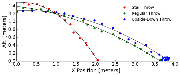
I'll use the Tracker video analysis software for this. We read in the video, setup some coordinate systems, markers, etc, and let it churn. If the frisbee veers in the third dimension (into or out of the screen) we won't get that information because we are just tracking its center in a 2D picture. Hence, I'll try to keep the throws gentle! We'll look at the stall, upside-down, and normal throws:
To keep this short, I'll tell you that the forward speed of these throws looks to top out at about 5 m/s. Again, we could go down the hole of getting drag from the slight deceleration in forward speed with time, but it really doesn't slow us much... the ground beats drag to stopping our frisbee.
We can see that the stall throw drops very quickly without really flying. In fact, it mostly is flipping end-over-end. The regular and upside-down throws look like they have a similar flight profile from the video. This means I must have not been as consistent as I had hoped with my throwing strength. We know that without the lift component that the upside-down throw should follow a more parabolic path than the regular throw. Also, my regular throw was pretty weak to keep the frisbee in the frame and minimally veering, so it didn't have enough lift to show us long periods of stable flight.
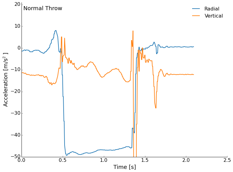
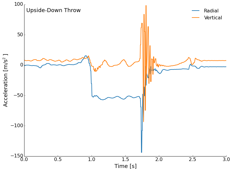
Next, let's look at the accelerometer data. The data is stored in a text file with the millisecond time stamp, and then each of the three axes acceleration measurements. I've plotted the radial (outward from the center) and vertical accelerations. Since the accelerometer was mounted near the rim of the frisbee, we will see relatively large signals from the wobble in flight.
We'll start with the normal throw this time. The accelerometer is roughly calibrated at the factory, but don't worry about the absolute values too much here. We see me pull back to throw as a upturn in the radial, then a large negative (outward) acceleration from the spinning of the disc during flight. Roughly a couple of g's here. The vertical is interesting through. We see the roughly -10m/s/s from the Earth's gravity as a prepare to throw and after the landing, but during flight we see a near zero vertical acceleration that trends downward. What is it? Lift! This is the flight of the frisbee that is gradually reduced as drag slows us and the angle of attack becomes non-ideal. We are expecting that we don't totally counteract gravity because flight is not sustained and our frisbee does not go on forever. This was a pretty gentle and short flight, but followed our expectations in terms of the forces at work. We can even see some precession in the vertical in the neighborhood of about 4 times/second.
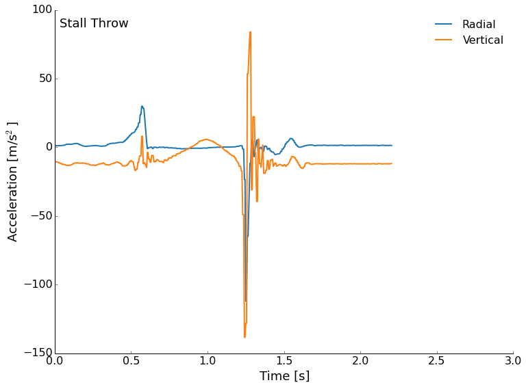
Next, we'll look at the stall throw. This isn't spinning so we don't expect to see a lot of radial acceleration once the throw leaves our hands, but we do expect to see some lift for a short period of time, then a stall and fall. That is what we get, too! The spike in the blue curve at 0.5 seconds is my push to accelerate the frisbee, then there are few other radial accelerations recorded (except the impact). There should be some small accelerations from the flip of the disc, but they are tiny here. The vertical trend up and down just before 1 second is the frisbee flipping over once. The only real lift is just a tiny fraction of a second before the front is lifted up. After that, we are really just in free-fall.
Finally, the elusive upside-down throw. The frisbee starts out upside-down, so the acceleration of gravity now shows as positive (look after the landing for example). We still see radial acceleration from the spinning and we also see a reduction in the vertical acceleration. This can't be lift, but is probably some axis mis-alignment on the sensor. We still see precession as the torque tries to keep the disc horizontal.
What did we learn?
We learned about all of the forces at play in the flight of a frisbee, lift, drag, etc. We measured some flight paths and acceleration profiles. These were not quite as clear cut as I had hoped though. We still saw that flying right side up works pretty well, but upside down "flight" is basically spin-stabilized falling with a lot of forward momentum. Throwing with no spin quickly results in a pitch-up and stall.
We'll see what happens with this. If people are interested we could think about adding an IMU to the setup with better positioning and balance. We could also just put a light on a frisbee and track it with a time-lapse photo. This turned out to be a fascinating look at flight, acceleration measurement, and video tracking! If you are wondering about numerical modeling, there is a really nice report from MIT that develops a good model.
#include <SPI.h>
#include <SD.h>
#include <Wire.h>
#include <Adafruit_Sensor.h>
#include <Adafruit_ADXL345_U.h>

/* Assign a unique ID to this sensor at the same time */
Adafruit_ADXL345_Unified accel = Adafruit_ADXL345_Unified(12345);

const int chipSelect = 4;

File dataFile;

void displaySensorDetails(void)
{
sensor_t sensor;
accel.getSensor(&sensor);
Serial.println("------------------------------------");
Serial.print ("Sensor: "); Serial.println(sensor.name);
Serial.print ("Driver Ver: "); Serial.println(sensor.version);
Serial.print ("Unique ID: "); Serial.println(sensor.sensor_id);
Serial.print ("Max Value: "); Serial.print(sensor.max_value); Serial.println(" m/s^2");
Serial.print ("Min Value: "); Serial.print(sensor.min_value); Serial.println(" m/s^2");
Serial.print ("Resolution: "); Serial.print(sensor.resolution); Serial.println(" m/s^2");
Serial.println("------------------------------------");
Serial.println("");
delay(500);
}

void displayDataRate(void)
{
Serial.print ("Data Rate: ");

switch(accel.getDataRate())
{
case ADXL345_DATARATE_3200_HZ:
Serial.print ("3200 ");
break;
case ADXL345_DATARATE_1600_HZ:
Serial.print ("1600 ");
break;
case ADXL345_DATARATE_800_HZ:
Serial.print ("800 ");
break;
case ADXL345_DATARATE_400_HZ:
Serial.print ("400 ");
break;
case ADXL345_DATARATE_200_HZ:
Serial.print ("200 ");
break;
case ADXL345_DATARATE_100_HZ:
Serial.print ("100 ");
break;
case ADXL345_DATARATE_50_HZ:
Serial.print ("50 ");
break;
case ADXL345_DATARATE_25_HZ:
Serial.print ("25 ");
break;
case ADXL345_DATARATE_12_5_HZ:
Serial.print ("12.5 ");
break;
case ADXL345_DATARATE_6_25HZ:
Serial.print ("6.25 ");
break;
case ADXL345_DATARATE_3_13_HZ:
Serial.print ("3.13 ");
break;
case ADXL345_DATARATE_1_56_HZ:
Serial.print ("1.56 ");
break;
case ADXL345_DATARATE_0_78_HZ:
Serial.print ("0.78 ");
break;
case ADXL345_DATARATE_0_39_HZ:
Serial.print ("0.39 ");
break;
case ADXL345_DATARATE_0_20_HZ:
Serial.print ("0.20 ");
break;
case ADXL345_DATARATE_0_10_HZ:
Serial.print ("0.10 ");
break;
default:
Serial.print ("???? ");
break;
}
Serial.println(" Hz");
}

void setup(void)
{
Serial.begin(9600);
Serial.println("Accelerometer Test"); Serial.println("");

/* Initialise the sensor */
if(!accel.begin())
{
/* There was a problem detecting the ADXL345 ... check your connections */
Serial.println("Ooops, no ADXL345 detected ... Check your wiring!");
while(1);
}

/* Set the range to whatever is appropriate for your project */
accel.setRange(ADXL345_RANGE_16_G);
// displaySetRange(ADXL345_RANGE_8_G);
//accel.setRange(ADXL345_RANGE_4_G);
// displaySetRange(ADXL345_RANGE_2_G);

/* Display some basic information on this sensor */
displaySensorDetails();

/* Display additional settings (outside the scope of sensor_t) */
displayDataRate();
//displayRange();
Serial.println("");
Serial.print("Initializing SD card...");
// make sure that the default chip select pin is set to
// output, even if you don't use it:
pinMode(SS, OUTPUT);

// see if the card is present and can be initialized:
if (!SD.begin(chipSelect)) {
Serial.println("Card failed, or not present");
// don't do anything more:
while (1) ;
}
Serial.println("card initialized.");

char filename[15];
strcpy(filename, "ACCLOG00.TXT");
for (uint8_t i = 0; i < 100; i++) {
filename[6] = '0' + i/10;
filename[7] = '0' + i%10;
// create if does not exist, do not open existing, write, sync after write
if (! SD.exists(filename)) {
break;
}
}

dataFile = SD.open(filename, FILE_WRITE);
if( ! dataFile ) {
Serial.print("Couldnt create ");
Serial.println(filename);
while(1);
}
Serial.print("Writing to ");
Serial.println(filename);
}

void loop(void)
{
/* Get a new sensor event */
for(int i=0; i < 100; i++){
sensors_event_t event;
accel.getEvent(&event);
dataFile.print(millis());
dataFile.print(",");
//log_float(event.acceleration.x,999,8,5);
dataFile.print(event.acceleration.x,5);
dataFile.print(",");
//log_float(event.acceleration.x,999,8,5);
dataFile.print(event.acceleration.y,5);
dataFile.print(",");
//log_float(event.acceleration.x,999,8,5);
dataFile.print(event.acceleration.z,5);
dataFile.println("");
}
dataFile.flush();
}
Ok, I've been sitting on this topic for awhile, but I was recently inspired to revive this post after being asked some very general questions by a tour group that came through the lab. Next time we'll be back to doing some data collection and analysis. Maybe gravity tide measurements? Anyhow, on with the topic of the day: knowing the fundamentals.
Rob quoted a line from the Windows 95 API Manual (a programming interface manual for the non-programmers out there). It said "The nature of an expert is not someone who knows all the details, it's someone who understands the fundamentals really well." Rob points out that therein lies the key to problem solving. This statement really resonated with me when I looked back on problems that I've encountered in the past, both scientific and technological.
We often think of an expert as someone that is in the top few percent of the knowledge leaders in their field. Experts should know all of the details of their subject, including the latest "bleeding edge" research right? While many experts do stay up to date, I began re-examining the people that I considered to be experts.
The professor may be the ideal example of this. While academics often get the connotation of the aloof and socially insulated genius, it's really not true. (In fact, our academic heroes are just people too, listen to the latest Nerds on Draft for that side story.) Professors have to teach the same material over and over again during their career. Sure, they should be pushing the frontiers of their field within their research group, but that's not what should be done in the education potion of the career. When you teach something, you end up deeply learning it yourself. In fact, that is part of the value in teaching! Be continually re-iterating the fundamentals to ourselves, we can stay primed to approach a new problem with a honed set of tools.
What could these fundamentals be? Well, that depends on your work. Maybe it is knowing the basics of programming or how to do basic chemical balance/thermodynamics calculations. Maybe it is knowing the fundamental operation of the product that you sell, or knowing the backstory to a concept you are helping someone with (such as the history of a topic).
I can't count the number of times that I've been trying to figure out a solution to a problem or how to build something when, after hours of no progress, something will make me start again. This time I look from a fundamentals viewpoint and can generally see a way to a solution or at least enough of the way to be able to ask an intelligent question.
Ideally, we are prepared for this way of problem solving by getting the basics of many fields during our undergraduate careers. Unfortunately that doesn't always happen. We have all sat in a math class, economics class, etc when the professor goes deep into a subject that they adore and leaves us in the dust. Another common occurrence is that the application of the fundamentals is not shown or sometimes not even implied. Not that students should be guided by the hand to the solution, but sometimes a firm nudge is necessary. I didn't necessarily appreciate this early in my undergraduate career, but later became a mass consumer of basic knowledge.
Next time you are on Amazon or in the library, browse over to a section with a topic of interest and pick up an introductory book. Read some sections, try some problems, and you'll be amazed at the other angles you can suddenly see as avenues of attack to a problem. You can even pickup some of your old text books and remind yourself of the fundamentals that all too often slip from our minds with time.
In the past on the "Don't Panic Geocast" we've talked about the speed of sound varying with temperature and how that can cause sound waves to bend. This phenomena, known as refraction, can result in all kinds of weird events, like being able to hear things from very far away when a thermal inversion is present in the atmosphere.
As I was researching some for that episode, I found that the standard formula for the speed of sound with temperature is a nice simple linear function over the ranges we care about. True, pressure and humidity can factor in there, but for simplicity, let's consider the largest factor... Temperature.
Formula for the speed of sound in dry air in m/s. Temperature is Celsius.
The formula above means that the speed of sound varies with temperature by 0.6 meters/second for every degree celsius of temperature change. That's about 2 ft/s for those of us more used to imperial units. A change that large should be pretty easy to see, right? This experiment and post were born from that statement.
To measure the speed of sound, I had several ideas. I could generate a short burst of noise and using an oscilloscope time how long it took to get to a microphone. That would require me to manually make the measurements, which probably means not a ton of data points since I'd have to either use the refrigerator to get a temperature difference or sit outside for a day. Neither of those were appealing. I ended up remembering some hardware that I had sitting around from the ultrasoniccave profiler.
The part of interest is the ultrasonic ranger. This little device (an SRF05) sends out a packet of ultrasonic pings and listens for their return. The device lets us know how long this takes by toggling an output from a digital 1 to digital 0. I already had the code to run this sensor, so I was half way there! The next thing I needed was a way to log the data. I didn't want to leave the door to the outside open to get power out there for the setup. I ended up using an SD card logger on top of the Arduino that was keeping track of the travel time.
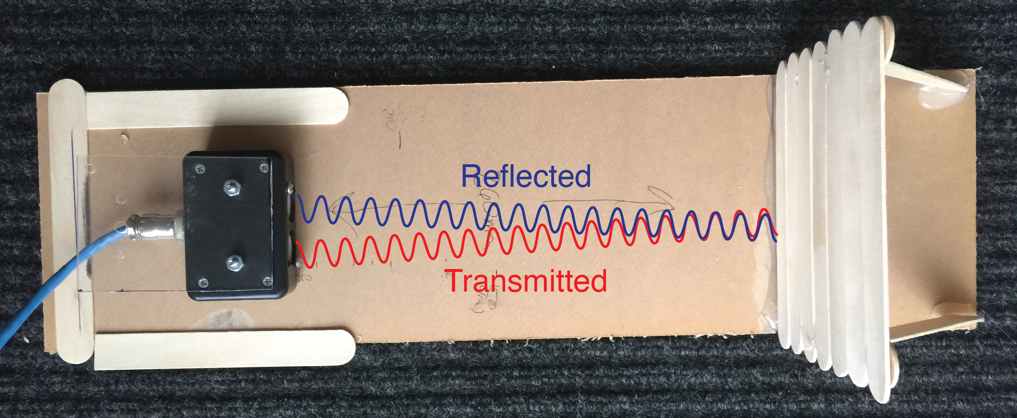
Finally, we needed a target to range. Luckily, this was easy to do with some wood sticks, hot glue, and a plexiglass base plate. I glued the target to the base 260mm from where the pinger was mounted. After a couple of quick tests, I had verified that the setup was working! Adding a temperature and humidity sensor to the breadboard gave us everything we needed. Time to collect some data!
Schematic of sound packets being transmitted and reflected. Really these are spherical wave-fronts, but the illustration is much cleaner this way!
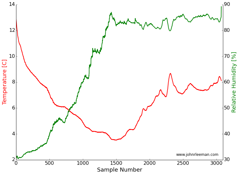
Luckily, we've had pretty wide temperature swings during the day here in Pennsylvania lately. Using a decent sized 12V battery and voltage converter I could get days of run time on a single charge. To get the best data possible, I averaged many travel times per sample. This took less than a minute to do, which is fine since temperature isn't changing that rapidly.
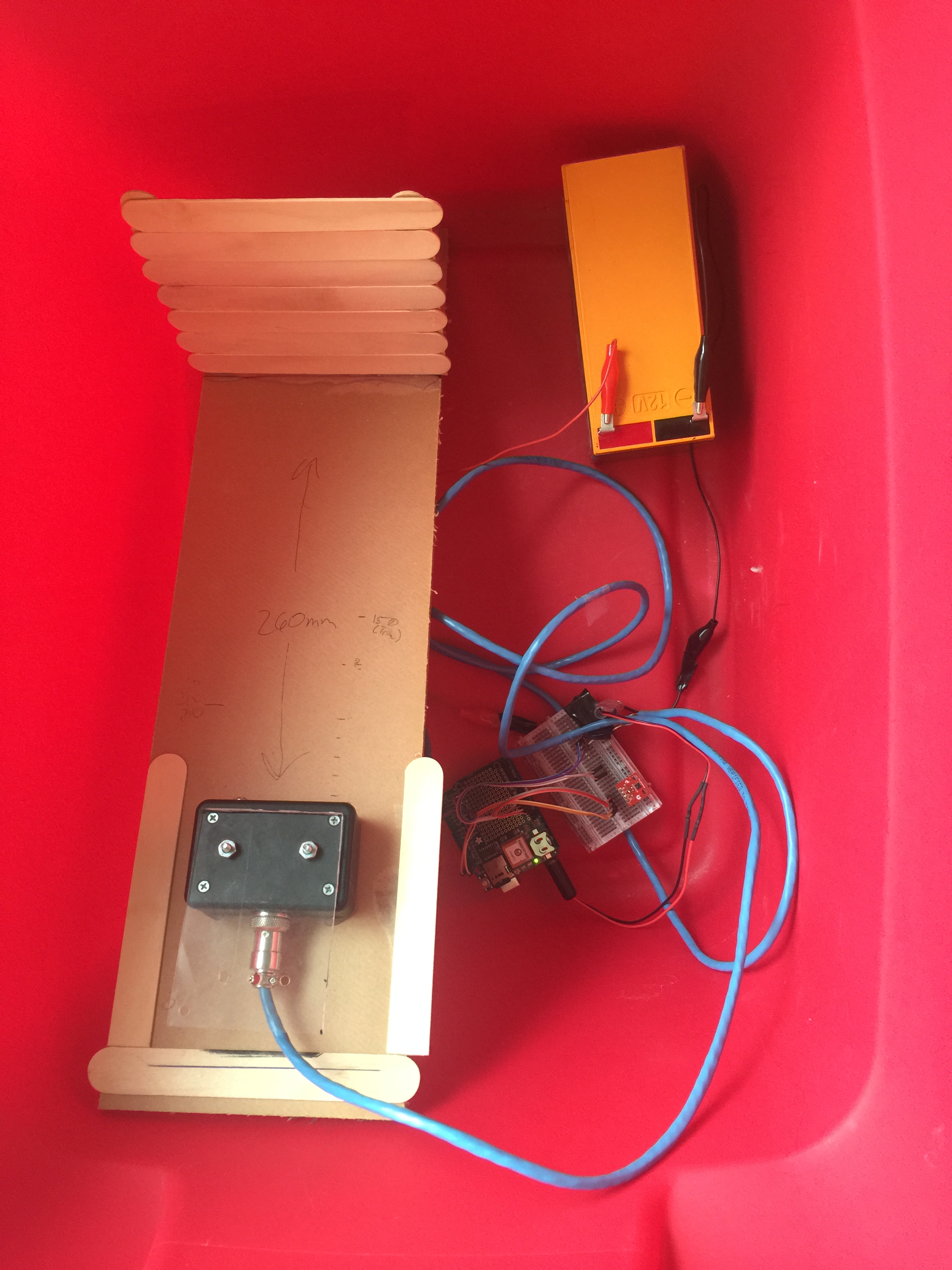
The complete setup in a tub ready to collect data outside.
Now that a simple apparatus was complete, I placed it in a Rubbermaid tub to keep any stray precipitation (or the rodents) from damaging things. The data was stored in a text file containing two-way travel time to/from the target in microseconds, device estimated distance to target, and the temperature/humidity readings. I collected several days worth of data, each time slightly improving my recording setup to get the cleanest data. I had problems with days where the temperature varied very fast and it appears to have introduced noise, some days there was direct sunlight (a rare thing in the PA winters) that caused very high temperatures and convection in the tub. Finally, on the last day of my experiment, I got a nice data set. It was a day with slowly varying temperatures and mostly cloudy. I trimmed the ends of the data so things were equilibrated and got some decent results!
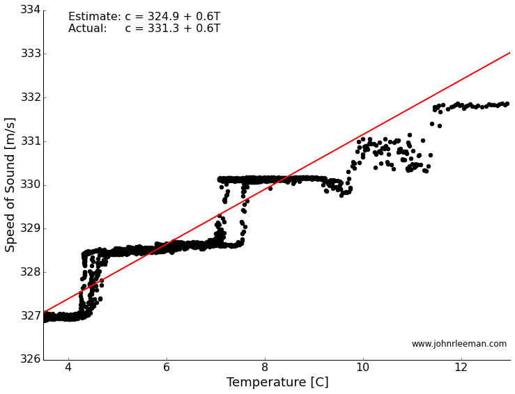
If we plot the temperature and the speed of sound against each other, we see what looks like a line! The steps are a result of being at the smallest increments in time that our system can sense. A better sensor could solve this, but for a rough estimate it turns out to be fine. Finding the best fit through this should tell us how well our measurements match the accepted formula. The slope of the line represents the rate of change of the speed with temperature (this should sound familiar to those calc. students out there), and the intercept represents the speed of sound at zero degrees.
We got the rate of change dead on! In fact we are within a few percent of the accepted value. The y-intercept is off by about 6 m/s, but I think that is a systematic offset due to a delay in the way the sensor is read. We could back that out, but maybe that is another topic for another time, or maybe we'll try this again with a different sensor. Please leave any comments or questions below!
This past week I got to relive some of my favorite days of primary education: the science fair! A local elementary school was hosting their annual science fair and had asked the department to provide some demonstrations for the parents and students to see. I immediately volunteered our lab group and began to gather up the required materials. Some of the setups were made years ago by my advisor. I also developed a few and improved upon others here and there. I thought it would be fun to share the experience with you.
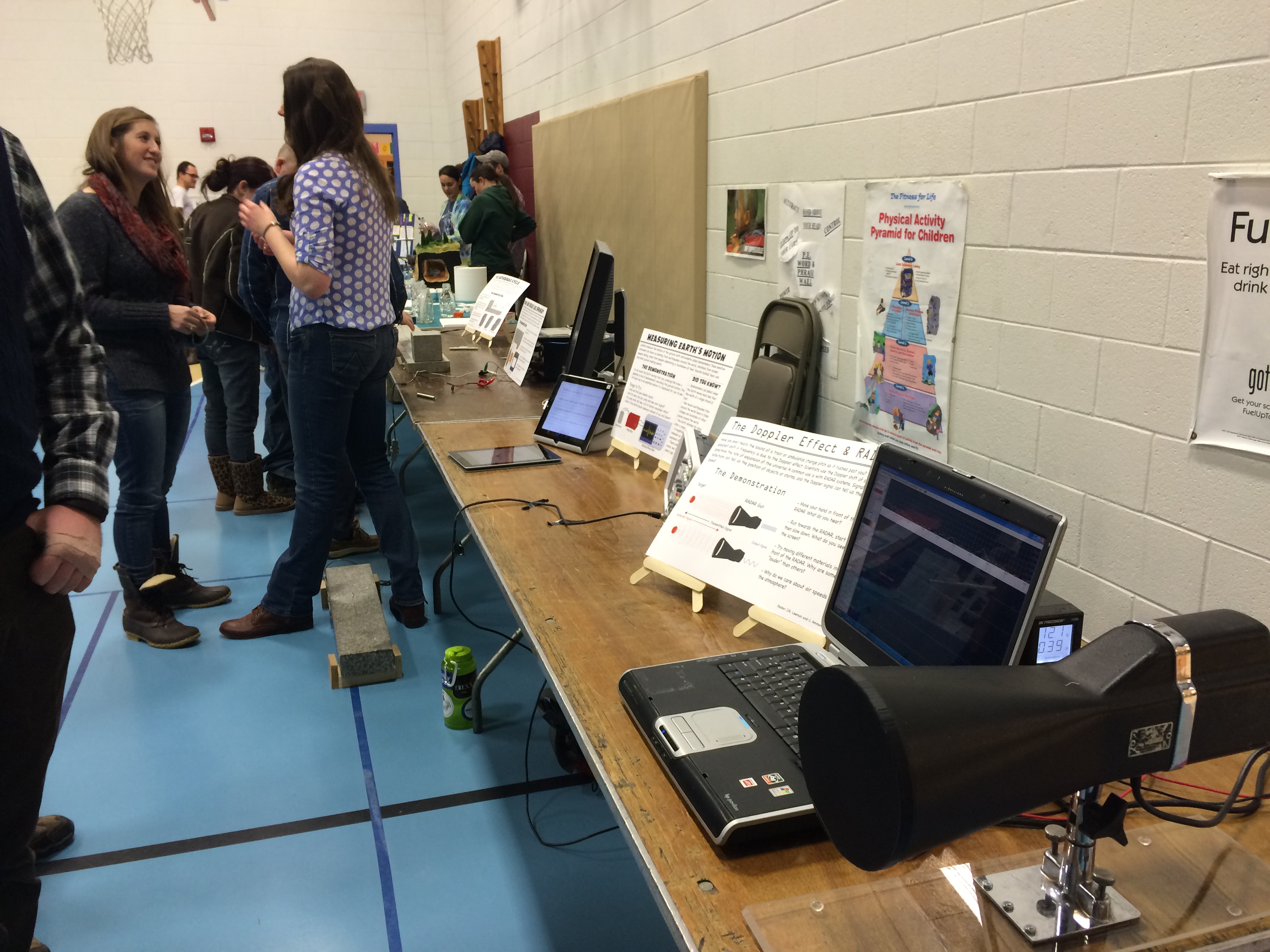
The line-up of demonstrations setup as the science fair was getting started.
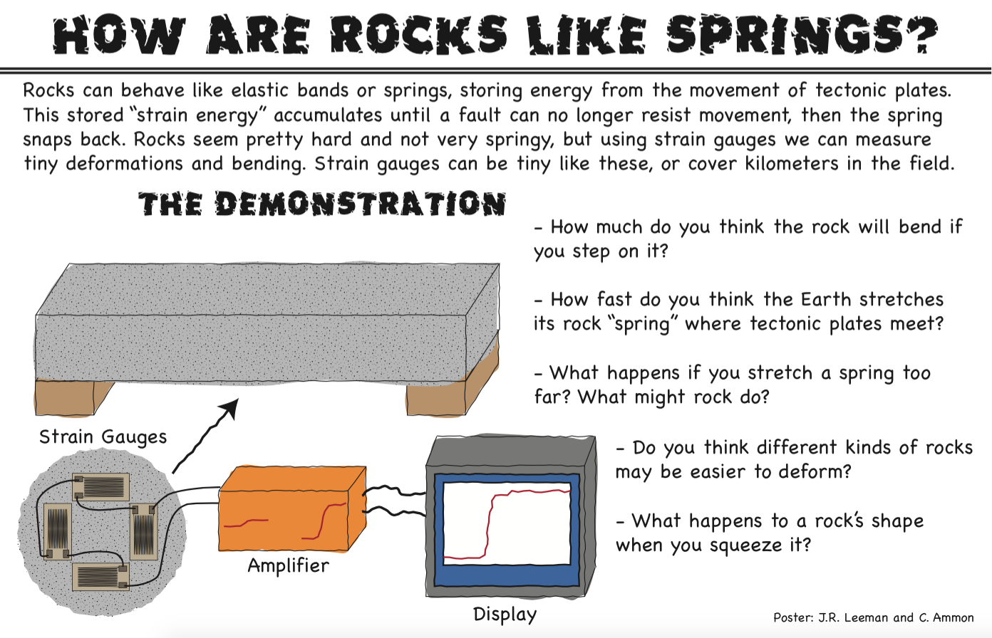
At some point, we should probably have a post or two about each of these demonstrations, but today we'll look at pictures and talk about the general feedback I received. First, off we had four demonstrations including the earthquake cycle, how rocks are like springs, seismometers, and Doppler RADAR. I made an 11x17" poster for each demo in Adobe Illustrator using a cartoon technique that one of our professors here shared with me.
Here is an example poster from one of the demonstrations.
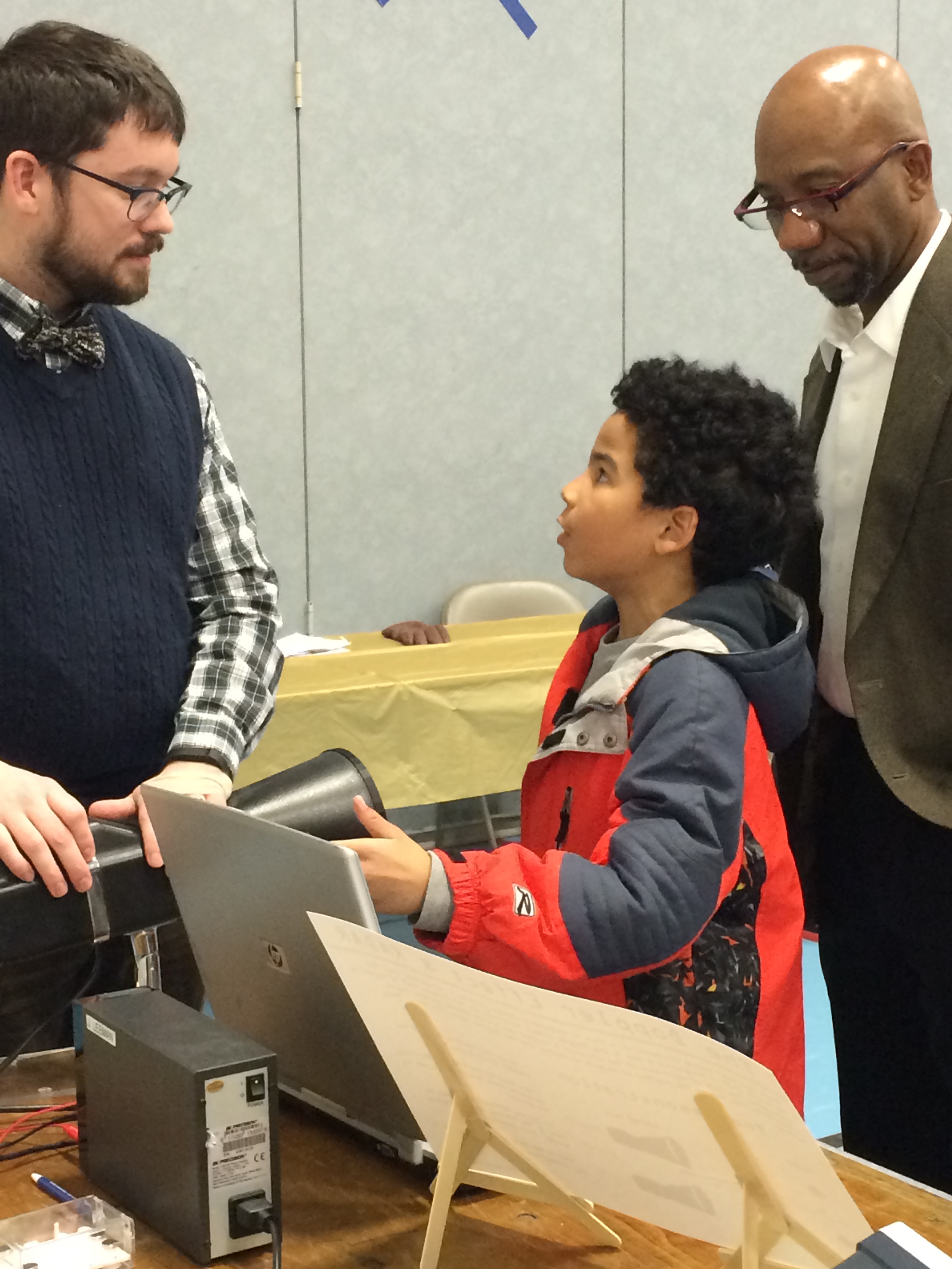
For scientists, communicating with the public can be difficult. It's easy for us to get holed up in our little niche of work and forget that talking about a topic like power spectra isn't everyday to pretty much everyone. Outreach events like this present a great opportunity to work on those skills! This particular event was especially challenging for me because the children were K-5, much younger than I usually talk to. With high school students you can maybe talk about the frequency of a wave and not get too many lost looks, but not with grade-schoolers!
The other difficulty was adapting what are deep topics (each demo is an entire field of research, or several) to the short attention span we had to work with. Elementary school teachers are masters of this and I would love to get some ideas from them on how to work with the younger minds. I spent most of my time talking about the Doppler effect with the RADAR (it's the topic my lab mates were least comfortable with since we don't deal with RADAR at work generally). By the end of the science fair, I had an explanation down that involved asking the kids to wave their hand slowly and quickly in front of the RADAR and listen to how the pitch of the output changed. Comparing that to the classic example of the pitch bending of a passing fire truck siren seemed to work pretty well. I had a "waterfall" spectra display that showed the measured velocity with time, but other than trying to get the line to go higher than their friends, it didn't get much science across (though lots of healthy competition and physical exercise was encouraged).
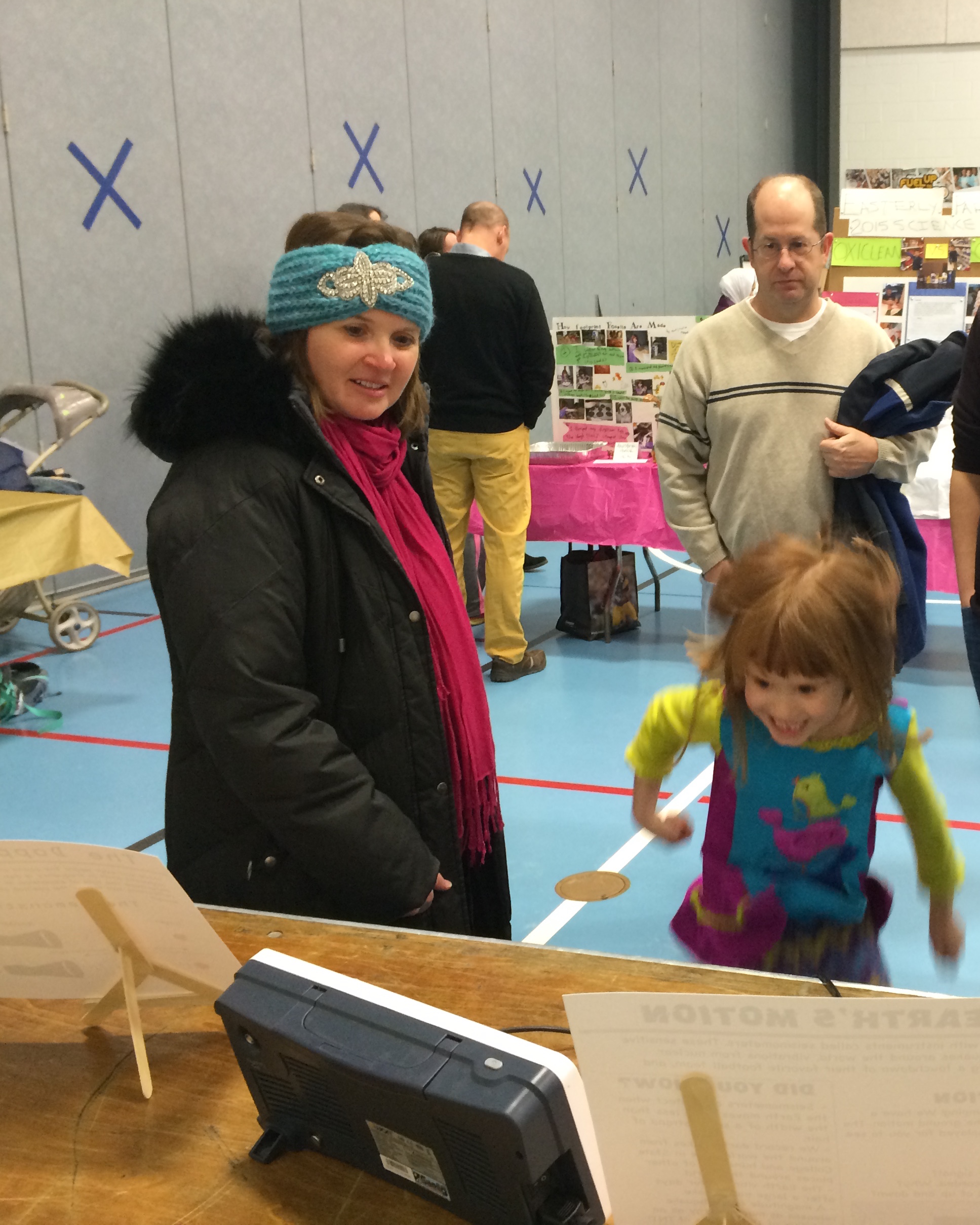
An excited student jumps up and down to see herself on a geophone display.
In the past, I've pointed out the value of being an "expert generalist". All of us were tested in any possible facet of science by questions from the kids and their parents. I ended up discussing gravitational sling-shot effects on space probes with a student and his parents who were incredibly interested in spaceflight. I also got quizzed about why the snow forecasts had been so bad lately, when the next big earthquake would be, and a myriad of other questions. Before talking to any public group, it's also good to make sure you are relatively up-to-date on current events, general theory, and are ready to critically think about questions that sound deceptively simple!
The last point I want to bring up today is the idea of comparisons. These are numbers that one of my committee members likes to say he "carries around in his shirt pocket." These are numbers that let us, as scientists, relate to others that are non-specialists and give us some physical attachment to a measurement. What do I mean? Let's say that I tell you that tectonic plates move anywhere from 2-15 cm/year. Great, first, since we are in the U.S.A., everyone will hold out their fingers to try to get an idea of what this means in imperial units.... not quite 1-6 in/year. That's better, but a year is a long time and I can't really visualize moving that slowly since nothing I'm used to seeing everyday is that slow... or is it? Turns out that fingernails, on average, grow 3.6 cm/year and hair grows about 15 cm/year. Close enough! In Earth science we have lots of approximate numbers, so these tiny differences are not really that bad. Now let's revise our statement to the kids to say: "The Earth is made of big blocks of rock called plates. These move around at about the speed your finger nails or hair grow!" Now it is something that anyone can relate to, and next time they clip their nails or get a hair cut, they just might remember something about plate tectonics! It's not about having exact figures in the minds of everyone, it's about providing a hand-hold that anybody can relate to! This deserves a post to itself though.
That's all for now, but I'd love to hear back from anyone who has elementary education experience or has their own "shirt pocket numbers."