When you hear "radar", you probably think of weather radar and a policeman writing a ticket. In reality there are many kinds of radar used for everything from detecting when to open automatic doors at shops to imaging cracks in concrete foundations. I've always found radar and radar data fascinating. Some time back I saw Dr. Gregory Charvat modify an old police radar on YouTube and look at the resulting signal. I happened to see that model of radar (a 1970's Kustom Electronics) go by on EBay and managed to buy it. I'm going to present several experiments with the radar over a few posts. If you want to learn more about radar and the different types of radar I highly recommend Dr. Charvat's book Small and Short-Range Radar Systems. I haven't bought a personal copy yet, but did manage to read a few chapters of a borrowed copy.
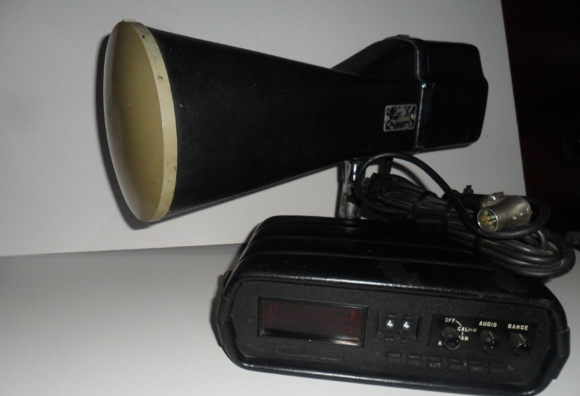
The doppler radar I purchased. I'm not using the head unit.
The radar I have outputs the doppler shift of a signal that is transmitted, reflected, and received. Doppler is familiar to all of us as we hear the tone of a train horn or ambulance change as it rushes past us. Since there is relative motion of the transmitter (horn) and receiver (your ears), there is a shift in received frequency. Let's say that the source emits sound at a constant number of cycles per second (frequency). Now let's suppose that the distance between you and the source begins to close quickly as you move towards each other. The apparent frequency will go up because the source is closer to you each emitted cycle and you are closer to the source!
The doppler effect of a moving source. Image: Wikipedia
This particular radar transmits a signal at a frequency of 10.25 GHz. This outgoing signal is continually transmitted and reflected/scattered off of objects in the environment. If the object isn't moving, the signal returns to the radar at 10.25 GHz. If the object is moving, the signal experiences a doppler shift and the returned frequency is higher or lower than 10.25 GHz (depending on the direction of travel). This particular radar can be easily hacked and we can record the doppler frequency out of a device called a mixer. The way this unit is designed, we can't tell if the frequency went up or down, just how much it changed. This means we don't know if the targets (cars) are coming or going, just how fast they are traveling. Maybe in a future set of posts, we'll build a more complex radar system such as the MIT Cantenna Radar. Be sure to comment if that's something you are interested in.
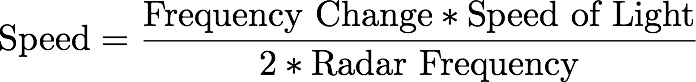
Since we'll be measuring speeds that are "slow" compared to the speed of light, we can ignore relativistic effects and calculate the speed of the object knowing the frequency change from the mixer, and the frequency of the radar.
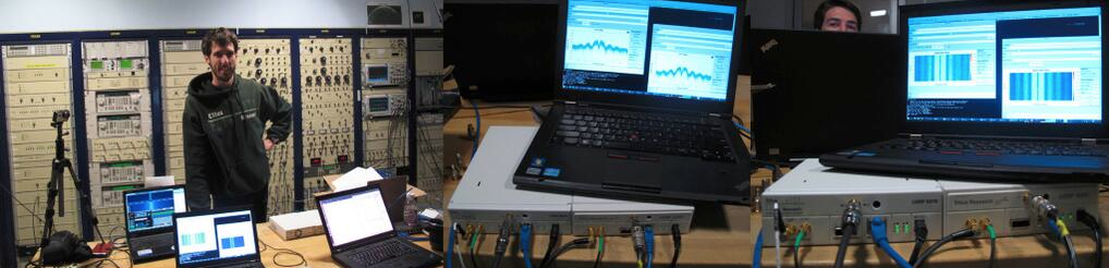
I took the radar out to the street and recorded several minutes of traffic going by, including city busses. Making a plot of the data with time increasing as you travel left to right and doppler frequency (speed) increasing bottom to top, we get what's known as a spectrogram. Color represents the intensity of the signal at a given frequency at a certain point in time.
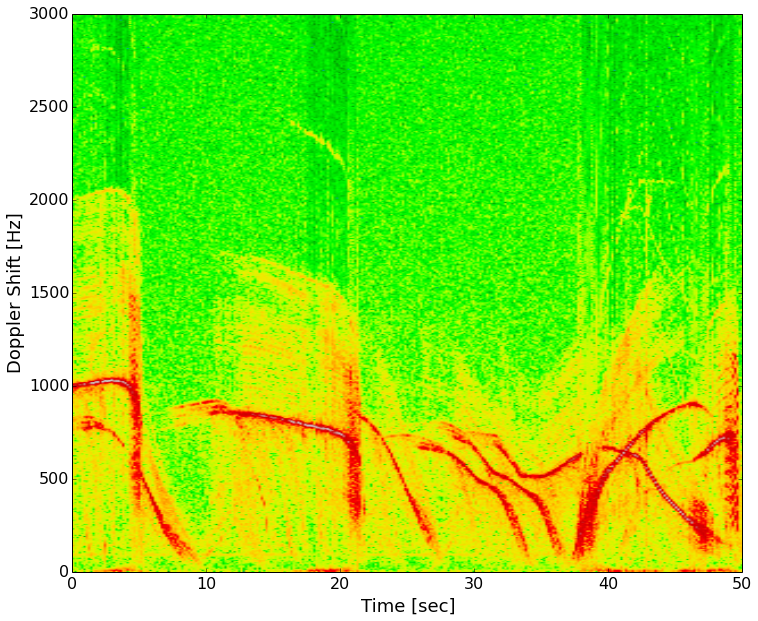
Speeds of several cars on my street. 1000 Hz is about 33 mph and 500 Hz is about 16 mph.
The red lines are strong reflectors (the cars). Most of the vehicles slow down and turn on a side street in front of the radar. About 30 seconds in there are three vehicles, two slow down and turn, the third again accelerates on past. Next I'll be lining up a video of these cars passing the radar with the data and you'll be able to hear the doppler signal. To do that I'm learning how to use a video processing package (OpenCV) with Python.
In the next few installments, we'll look at videos synced with these data, radar signatures of people running, how radar works when used from a moving car, and any other good targets that you suggest!