Category Archives: General Science

Raindrops Keep Falling on my Radar - Part 2

Last time we looked at the raindrop fall speed of raindrops during a thunderstorm and compared the radar reflected power to my observations of the storm moving through State College. Today, thanks to Yvette Richardson and Bill Syrett from the Penn State Meteorology Department, we can compare the radar returns to actual weather station data. They were able to provide data from a weather station on top of the meteorology building on campus, about 3 miles from where my radar was located.

We expect more power to be returned to the radar during periods of heavy rain, so the main variable of interest is the rain rate. We'll plot up a couple of other meteorological variables just for fun as well. The weather station recorded observations every minute. I had to venture my best guess at the units based on their values. The rain rate values are low. Another station that I don't have the time-series for reported a maximum rain rate of 0.26 in/hr. Either way, let's examine the relative changes.

rain_wx_data_graph


Looking at the plot we can see that our prediction of higher rain rate equaling more reflected power holds. Unfortunately, the weather station didn't record precipitation rate with very fine resolution, so we really can only match the peak rain rate with the peak reflected power. The vertical red line marks the time of a weather service doppler radar screenshot we looked at in the last post that was right before the heaviest rain arrived. We also observe the higher wind speeds with the gust front ahead of the storm. As the storm passed over we saw decreasing pressures as well. The temperature and humidity aren't shown because they really weren't that interesting.

Now that we've verified our hypothesis (roughly anyway) about precipitation rate and radar return, we are ready to look at different types of reflectors. Next time, we will look at radar data collected during a snow storm for return intensity and the fall speed of snow flakes. That speed can be compared with video of falling snow for verification. Stay tuned!

Raindrops Keep Falling on my Radar - Part 1

What's the most complicated way to say it's raining? Well, if you know me, you know it will involve electronics, sensors, and signal processing! This post was originally going to compare the fall velocity for rain, sleet, and snow. Unfortunately, I haven't been lucky enough to be home to run my radar when it was snowing. It will happen this winter, but we'll start looking at some data now. Want to review radar before we get started? We have already talked about looking at the doppler signature of cars and got a tour of a mobile weather radar.

Back in October we had a couple of squall lines come through. On the 3rd, there was a significant event with two lines of storms. I had just been experimenting with measuring rainfall velocity with the modified X-band radar, so I decided to try another experiment. I put the radar unit in a trashcan and covered it with plastic bags. Then I sat it outside on our balcony and recorded for about 2.5 hours.

Testing the radar setup before the rain with some passing cars as targets.

Testing the radar setup before the rain with some passing cars as targets.

There is a radar in there! My make-shift rain proof radome. The only problem was a slight heat buildup after several hours of continuous operation.

There is a radar in there! My make-shift rain proof radome. The only problem was a slight heat buildup after several hours of continuous operation.

Not only do we get the doppler shift (i.e. velocity of the raindrops), but we get the reflected power. I'm not going to worry about calibrating this, but we can confidently say that the more (or larger) raindrops that are in the field of view of the radar, the more power will be reflected back.

First, let's look at a screenshot of the local weather service radar. You can see my location (blue cross) right in front of the second line of showers. At this point we had already experienced one period of heavy rain and were about to experience another that would gradually taper off into a very light shower. This was one of the nicer systems that came through our area this fall.

A capture of our local weather radar, my location is the blue cross directly ahead of the storm.

A capture of our local weather radar, my location is the blue cross directly ahead of the storm.

Now if we look at the returned power to the radar over time, we can extract some information. First off, I grouped the data into 30-second bins, so we calculate the average returned power twice per minute. Because of some 32-bit funny business in the computations, I just took the absolute value of the signal from the radar mixer, binned it, and averaged.

Reflected power received by the radar over time. The vertical red line is the time that the radar screen shot above was taken.

Reflected power received by the radar over time. The vertical red line is the time that the radar screen shot above was taken. We can see the arrival and tapering off of the storms.

From this chart we can clearly see the two lines of storms that came over my location. We also see lots of little variations in the reflected power. To me the rain-rate seemed pretty constant. My best guess is that we are looking at skewing of the data due to wind. This could be solved with a different type of radar, which I do plan to build, but that doesn't help this situation.

Let's look at what inspired this in the first place, the rainfall velocity. From a chart of terminal velocities, we can see that we expect to get drops falling between 4.03-7.57 m/s for moderate rain and 4.64-8.83 m/s for heavy rain. Taking a 5 minute chunk of data starting at 60 minutes into the data (during high reflectivity on the chart above), we can compute the doppler frequency content of the signal. Doing so results in the plot below, with the velocity ranges above shaded.

psd_velocity

Doppler frequency content of 5-minutes of data starting at 60 minutes into recording. The blue box shows doppler frequencies corresponding to moderate rain, and the red box corresponding to heavy rain.

Based on what I see above, I'd say that we fall right in line with the 0.25"-1" rain/hour data bracket! There is also the broad peak down at just under 100 Hz. This is pretty slow (about 1 m/s). What could it be? I'm not positive, but my best guess is rain splattering and rebounding off the top of my flat radar cap. I'm open to other suggestions though. Maybe part of this could be rain falling of the eve of the building in the edge of the radar view? The intensity seems rather high though. (It was also suggested that this could be a filter or instrument response artifact. Sounds like a clear air calibration may help.)

So, what's next? We'll take some clear-air calibration data and the use data from a Penn State weather station to see what the rain rate actually was and what the winds were doing. Maybe we can get a rain-rate calibration for this radar from our data. See you then!

Thank you to Chuck Ammon for discussions on these data!


Don't Panic Geocast - Now on Your Radio!

DSCF4046

I would like to announce the official release of the first episode of the "Don't Panic Geocast!" This is something that has been in the works since earlier this summer. Each week Shannon Dulin and I will be discussing geoscience (geology, meteorology, etc) and technology. Please be sure to add us to your feeds and checkout our first show!

Breaking the Wishbone - How to Win

The folks over at Michigan Engineering did some modeling, 3D scanning, and experimentation to tell us how to win at the age-old Thanksgiving game of breaking the wishbone. According to the folks over at aaepa.com, the tradition is much older than Thanksgiving, dating back over 2400 years to cultures that believed that birds were capable of telling us the future. There is even suggestion that the phrase "getting a lucky break" can be traced to this tradition.  If you want to win, watch the 76 second video below and remember: choke up, stay stationary, and pick the thick side.

We Are ... Seismic Noise

2014-10-28 13.27.05

Over the last few months construction crews have been hard a work tearing into the building adjacent to mine on the Penn State campus. Lots of demolition has been happening as the old building is completely cleaned out and being rebuilt. Some of the noise has been so strong that we could feel it next-door. As a data-nut, my first thought was "I'm going to look at this on our seismometer!"

At the base of Deike building (the geoscience building), we have a seismometer. The station, WRPS "We aRe Penn State", has been in operation on an isolated pier for some time, so we have lots of data to look at! For our purposes, I downloaded the entire month of October for 2013 and 2014. There are some hours/days that are missing, but we'll ignore those and work with what we have. This is a common problem in geoscience!

First let's just make a plot of this year's data. Each square represents one hour (24 squares in a row), and each row represents one day. Missing data is the lightest shade. The squares are colored by the strength of the seismic energy received during that hour; the darker the square, the more energy received.

WRPS_2014_HourlyYou'll immediately notice that there is always more noise starting about 11 UTC, which is the 7-8 AM hour locally. This is about when people are coming into work, vibrating the ground and buildings on campus as they do. The noise again seems to die off about 21 UTC or the 5-6 PM hour locally. This again makes sense with people leaving work and school. This isn't split finely enough to look for class change times on campus, but that could always be another project.

The other thing to point out is the dates of October 4-5,11-12,18-19,25-26. These are the weekends! You notice there is less of the normal daily noise traffic with fewer people on campus and construction halted. There is a repeating noise event at 11 UTC on the 1st, 12th, 20th, and 27th. I'm not sure what that is yet, but looking at more months of data may indicate if that event is associated with equipment starting up, or is really random.

While these daily life trends are interesting, they have been observed before. This whole discussion started with construction and how it was affecting the noise we saw on our local station. To examine this, I made a stacked power spectral density plot. Basically, this shows us how much energy is recorded at different frequencies. The higher frequencies would be human activity.

WRPS_PSD

We can see that the curves from 2013 and 2014 are very similar, with the exception of the 11-16 Hz range. In that range, the energy is higher in 2014 than in 2013 without construction by about a factor of 10. That range makes sense with construction activity as well! The energy remains elevated even after the main bump out to 20 Hz.

You might be thinking that such a bump could be due to anything. That's not necessarily true considering that we have stacked a month's worth of data for each curve. To show how remarkably reproducible these curves are, I made the same plot for the same times with a station in Albuquerque, New Mexico.

ANMO_PSD


In the Albuquerque plot, the two years are very similar, nothing like the full order of magnitude difference we saw in University Park. There are obviously some processing effects near 20Hz, but those are not actual signal differences, just artifacts of being near the corner frequency.

That's it for now! If there is interest, we can keep digging and look at signals resulting from touchdowns in football games, class changes, factories, etc. A big thank you to Professor Chuck Ammon as well for lots of discussion about these data and processing techniques.

315 Million Miles From Home, Cold, and Landing on a Ball of Ice

Rosetta's_Philae_touchdown

Image: Wikimedia

Tomorrow (November 12, 2014), the Philae robotic lander will detach from the parent spacecraft, Rosetta, and begin its short trip to the surface of comet 67P/Churyumov–Gerasimenko. This is a big step in technology and spaceflight! I'm sure we'll hear lots of fascinating new discoveries in the coming weeks, but before the lander detaches I wanted to point out how amazing this mission already is and a few things that it has already taught us.

First, let's talk about distance and speed. Space often confounds us with mind-boggling distances, sizes, and speeds. Rosetta was launched in 2004 and made a few loops in the inner solar-system to use gravitational acceleration to help it get out past Mars. As of this writing, Rosetta was about 315 million miles away from Earth, having actually travelled much further (map below). It is orbiting a small body (a comet) that is traveling at about 44,700 miles per hour (20 km/s). It is also orbiting very low to the comet, only about 19 miles (30 km) off the surface.

Image: ESA

Image: ESA


In the morning, at about 3:35 AM Eastern Time, the Philae probe will detach from the orbiter and begin the seven hour journey to a landing on the comet's surface. Not only is landing on a moving target far from home difficult, but it is made even more difficult by the small size of the comet. We know that small bodies exert less gravitational attraction on other objects (it's directly proportional to the mass if you remember the Law of Gravitation). Small masses are normally good, because it means that we don't have to be going as fast to escape the gravitational influence of the planet. For example, the escape velocity of Earth is about 25,000 miles per hour (11.2 km/s), while the escape velocity of the moon is only about 5,400 miles per hour (2.4 km/s). The escape velocity of the comet is only about 1.1 miles per hour (0.5 m/s)! Since the spacecraft is descending at about 1 m/s, this presents a problem: it would likely touch the comet, then bounce off, never to be seen again.

To solve the landing problem, Philae has legs with a strong suspension system that utilizes the impact energy to drive ice-screws into the surface. For additional security, two harpoons will be fired into the surface as well.

One of the ice drills securing the lander. Image: Wikimedia

One of the ice drills securing the lander. Image: Wikimedia


Once on the comet, the suite of 10 instruments will begin to collect data about the magnetic field, composition, and other parameters. I'm sure the team will have many fascinating discoveries to share, but in the interest of keeping this post short, I'd like to share one result we already have.

Rosetta has been, and will continue, to collect data from orbit with radar units, cameras, magnetometers, and spectrometers. As Rosetta began to get close, scientists noticed a periodic variation in the magnetic field around the comet. These variations are very low in frequency, about 40-50 milli-Hertz. We can't hear anything that low in frequency, but if you artificially bump up the frequency so we can listen to the data, you get the following:

What is most fascinating about this is that it was totally unexpected! Scientists are unsure of the cause. This is one of the many puzzles that Rosetta and Philae will reveal, along with a few of the answers. Best of luck to the team. We'll check in on the spacecraft again in the future and see what we've learned.

One last note: even traveling at the speed of light, the radio signal confirming the spacecraft status will take about 30 minutes to travel from Philae to us! Be sure to watch live tomorrow (here).


Doppler On Wheels - A Tour of a Mobile Radar

DOW7_Web

Recently, Penn State was lucky enough to have the "Doppler on Wheels" or DOW visit for two weeks through an NSF education grant! The truck, owned and operated by the Center for Severe Weather Research, is probably familiar to you if you have watched any of the storm chasing television shows or are interested in severe storms.  Dr. Yvette Richardson and Dr. Matt Kumjian were the faculty hosts and incorporated the radar into classes they are teaching.

I've always believed in getting students involved with data collection.  If students collect the data, they are attached to it and begin to see the entire scientific process.  Data doesn't just appear, real data is collected, often with complex instruments, and processed to remove various problems, corrections, etc.  It's not everyday that students get to collect data with a state-of-the-art radar though!

For this entry we're going to try a video format again.  Everyone seemed to like the last video entry (Are Rocks like Springs?).  Keep the feedback coming! It was a bit windy, but I've done what I can with the audio processing.  A big thanks to everyone who let me talk with them!  As always, keep updated on what's happening by following me on twitter (@geo_leeman).  This week I'll be off to New York to hear Edward Tufte talk about data visualization, so expect updates about that!

Fun Paper Fridays

Image: phdcomics.com

Image: phdcomics.com

In my last post about why I think the expert generalist is crucial in today's highly inter-related world, I mentioned a practice that I've adopted of "Fun Paper Fridays."  Today I want to briefly describe fun paper fridays and invite you to participate.

The Routine
Every friday I go to a coffee shop first thing in the morning and commence my weekly review.  During this time I check the status of projects, emails, etc and make sure that things are not slipping through the cracks.  Those of you familiar with David Allen's Getting Things Done will recognize this.  In addition to reviewing my schedule, I added a self expansion project.

Each week I pick out a paper that isn't directly related to my research and read it.  The paper can be serious, just not about my work (ex: Viking Lander 1 and 2 revisited: The characterization and detection of Martian dust devils), or it can be a completely fun topic (ex: How to construct the perfect sandcastle).  That's it! Just read a paper, no notes unless you want.  You'll be surprised when in some situation you'll recall a fact, method, or comment from one of these papers and be able to apply it to a completely different scenario.

Join Me
I hope that you'll join me in this quest of broadening your knowledge horizons. If you're not involved with science, that's no problem. Just read something that you normally wouldn't. Maybe it's the Art & Culture section of a newspaper or an Article from a popular science magazine. Every Friday I'll be posting the paper I'm reading on Facebook and Twitter. Please join me and use the tag: #FunPaperFriday.

NSF Graduate Fellowships - Some Thoughts and Tips

While this post may not appeal to the general audience, I thought it would be useful because it is an important topic to any senior undergraduate or first/second year graduate student. Today I want to briefly tell you my experience applying for the NSF Graduate Fellowship in 2012 and 2013.  I learned a lot in the process of applying for this prestigious fellowship and hope that I can pass some of that knowledge down!

Application 2012 - No award

My first year at Penn State, I applied with the traditional three documents of research statement, personal statement, and research proposal.  I sought the edits of those who had been awarded the fellowship in the past and thought I had a convincing packet assembled.  After reading, re-reading, and re-reading, it was time to submit.  I submitted the application, then made the mistake of reading over it again a week later and finding things I wished I had changed.  Months went by and seemed to drag on until the award announcements came.  I was not selected for an award.  While I was of course disappointed, it was time to kick it into high gear and make an even better application for my next (and final) try.

Application 2013 - Award Offered

For my second application I had lots of debates with myself.  Should I change my research proposal topic? Were my personal and research statements too similar? How can I improve the writing? Should I include figures?

To settle these debates, I turned to the wealth of online information that I hadn't sought out the previous year.  I talked with those who had received the award, I read funded research proposals from various professors and researchers, and I went down to the bare bones of the document.  While I'll discuss specific tips below, I'll just say that I started earlier, took more pauses between writing sprints, and sought more people for reading.

My tips

In writing two proposals, I learned a lot about how to effectively structure my research and emphasize the specific angle of attack I'll take on a research question and why it's different.  Here are some things I found to be helpful:

MY PROCESS

  • Start Early - Think it's too soon? Wrong! You need lots of time to organize your thoughts, revise, rewrite, and think about your application.
  • Read the Announcement - Print out the announcement document and read it critically.  You can look at the 2014 announcement here.  Don't just read it, mark on it. Highlight what they specifically are looking for, underline the buzzwords and key phrases of the call.  Also, draw a big box around the application deadline and then plan to beat it by one week.  Why? Computer problems, server crashes, unexpected medical emergency, etc.  You don't know what could happen, so make sure that your application gets in early!
  • Make a FastLane Account - Go to the online application and make an account.  Get familiar with FastLane, you'll use it for most all of your NSF proposals unless they change sometime in the future! Look at the application.  Go ahead and fill in the boxes with your name, address, etc.  Now you can mark down progress on your application and have momentum to move forward with the hard work.
  • Write the Requirements for your statements out on Paper - This one is huge.   In the application, pull up the research proposal and background/personal statement "prompts."  Print them, read them many times, and finally write them down on a notepad.  Break the prompt up into small chunks and then think about how to answer each piece.  Don't worry about flow, just think.
  • Brain Dump - Now write each one of the pieces of the question on the top of a page and begin to outline the points that you will make to address it.  Again, don't worry about order or how many points you have! Just write and write and write.
  • Organize into an Outline - Take a break, a day or so, then come back to your brain dump afresh and think about how you can piece it together into one coherent story - your story.  The story of a proposed research project and the story of you and your life in science.
  • Make a Draft - It does not need to be pretty, organized, the right length, etc.  Just get complete sentences onto the page.  Do this on paper or in a plain text editor.  Don't worry about formatting, length, spacing, margins... Those are things for later in a word processor.  I like using Textastic, Sublime, TextWrangler, or Editorial.
  • Read it and Have Lots of People Read it - Don't be afraid to ask everyone to read and edit your document.  Do not ask them to re-write the document for you! Remember this needs to come from your brain, but it is fine to gather suggestions and comments.  I also went to the graduate writing center and had some great suggestions from the coach there.  As scientists, we are not used to marketing ourselves and we often think the need for our research is obvious.... That won't work.
  • Talk to Your Reference Writers - You'll need letters of reference.  These take lots of time to write, so make things easy on your mentors and writers.  They have done a lot for you and are about to help out again.  I went through the application, figured out what I thought would be important to my application reviewers and then composed an email to my writers (see below).
  • Do NOT Cram - Whitespace is a dear friend to someone who is reading many pages of documents... like your judges.  Don't pack every single word you possibly can into the pages.  Economy of words shows great thought and restraint when writing.  Edit down over and over.  Leave white space between paragraphs.  If you use figures, text wrapping is a fine way to reclaim space, but leave a sufficient margin.  Look at books and other professionally formatted documents for inspiration.

MY APPLICATIONS FROM BOTH YEARS

Here are links to documents I produced for both applications, of course don't plagiarize, but hopefully they are helpful!

NSF 2012 (No Award)
Personal Statement | Previous Research | Proposed Research

NSF 2013 (Award Offered)
Research Statement | Personal & Background Statement |
Letter to Reference Writers

LINKS

There are several other helpful webpages out about the application process.  Remember, what you read on the program site is the final word, but these pages have more useful tips.

GRFP Essay Insights (Missouri)
Alex Lang's Website
Jennifer Wang's Website
Reid Berdanier's Website
The Official NSF GRFP Page
NSF PAPP Guide Book

Remember, if you don't get the award, take the feedback you get and start improving! Try, try again and don't be afraid to seek help from mentors, writers, friends, and family.  Please leave any useful comments below. Best of luck!

Mythbusting: Cooling a Drink with a Wet Paper Towel

While reading one of the many pages claiming to have "15 Amazing Life Hacks" or something similar, I found a claim about quickly cooling a drink that deserved some investigation.  The post claimed that to quickly cool your favorite drink you should wrap the bottle/can in a wet paper towel and put it in the freezer.  Supposedly this would quickly cool the drink, faster than just the freezer.  My guess is that the thought process says evaporative cooling is the culprit.  This is why we sweat, evaporating water does indeed cool the surface.  Would water evaporate into the cold, but dry freezer air? Below we'll look at a couple of experiments and decide if this idea works!

We will attack this problem with two approaches.  First I'll use two identical pint glasses filled with water and some temperature sensors, then we'll actually put glass bottles in and measure just the end result.  While the myth concerns bottles, I want to be able to monitor the temperature during the cooling cycle without opening the bottles.  For that we'll use the pint glasses.  

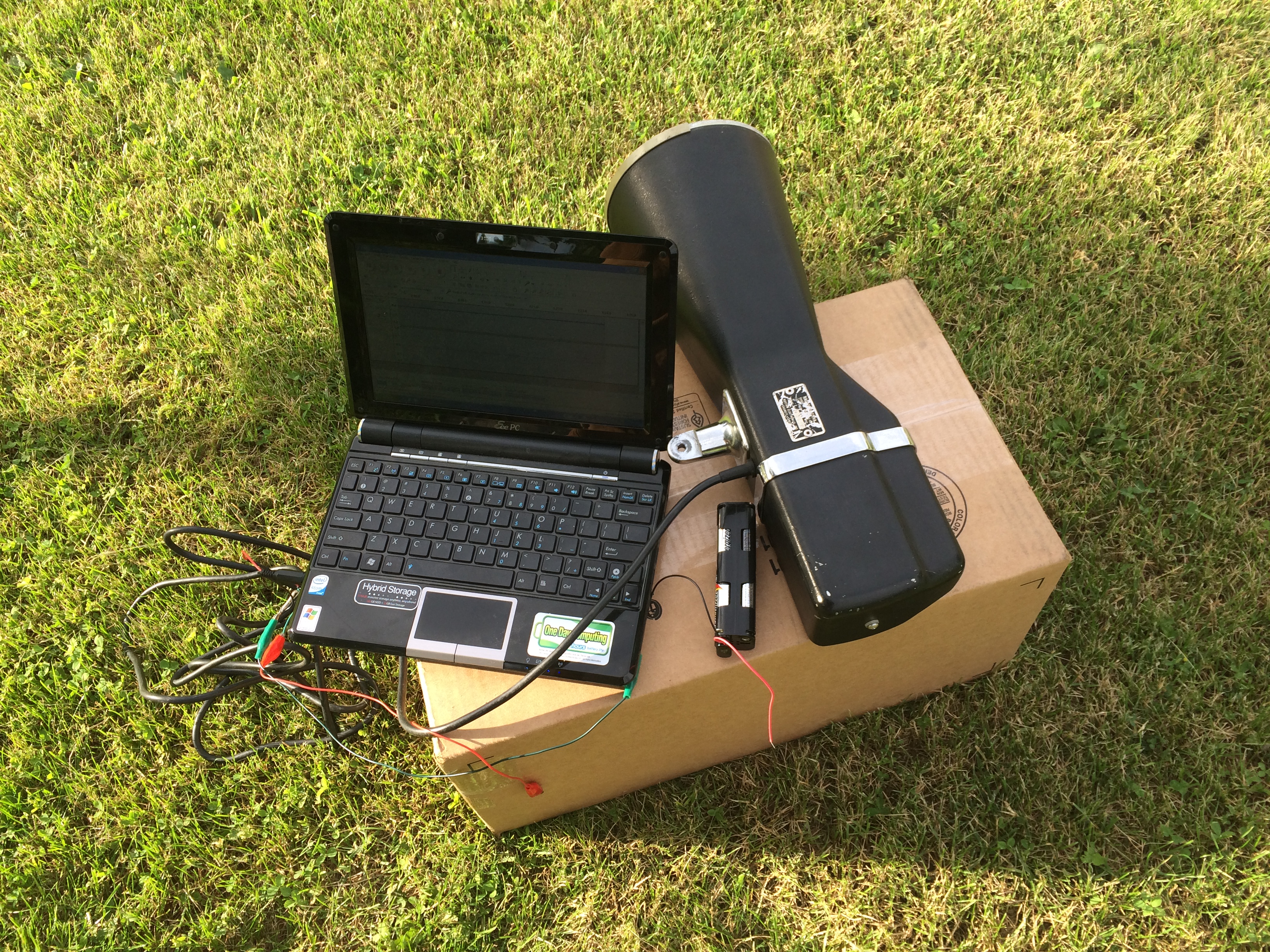
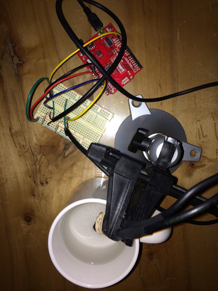
First I had to build the temperature sensors.  The sensors are thermistors from DigiKey since they are cheap and relatively accurate as well.  To make them fluid safe, I attached some three-lead wire and encapsulated the connections with hot-glue.  The entire assembly was then sealed up with heat-shrink tubing.  I modified code from an Adafruit tutorial on thermistors and calibrated the setup.  

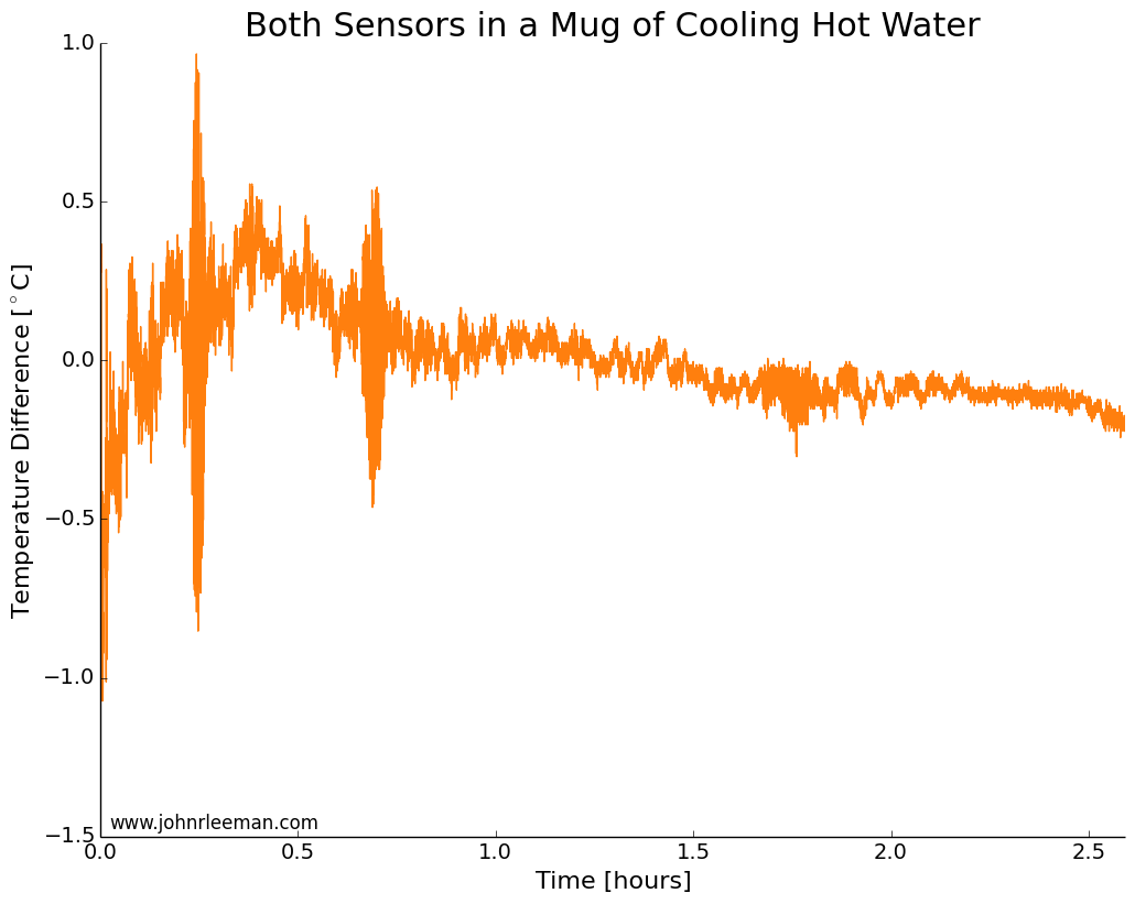
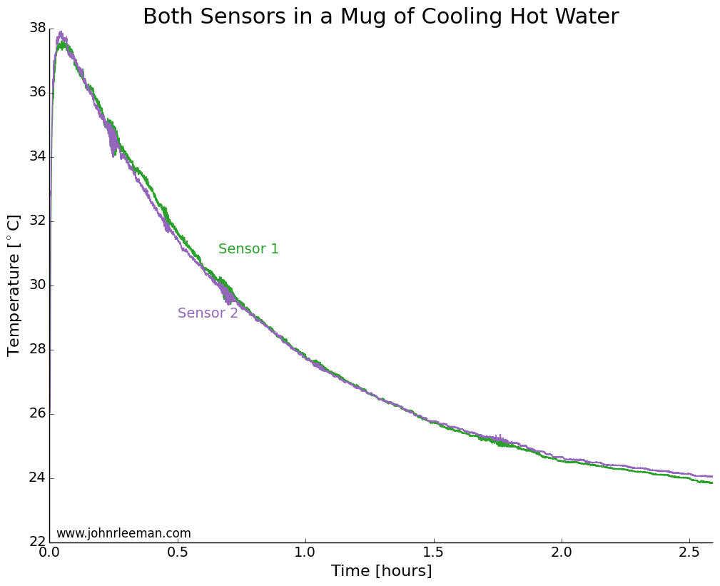
To make sure that both sensors had a similar response time, we need to do a simple control test.  I placed both probes in a mug of hot water right beside each other.  We would expect to see the same cooling at points so close together, so any offset between the two should be constant.  We also expect the cooling to follow a logarithmic pattern.  This is because the rate of heat transfer is proportion to the temperature difference between the water and the environment (totally ignoring the mug and any radiative/convective transfer).  So when the water is much hotter than the air, it will cool quickly, but when it's only slightly hotter than the air it will take much longer to cool the same amount.  

Mug Cooling Photo

Plotting the data, we see exactly the expected result.  Both sensors quickly rise to the water temperature, then the water cools over a couple of hours.  The noisy segments of data about 0.25 hrs, 0.75 hrs, and 1.75 hrs in are likely interference from the building air conditioning system.  

CoolingWater_AbsoluteTemps

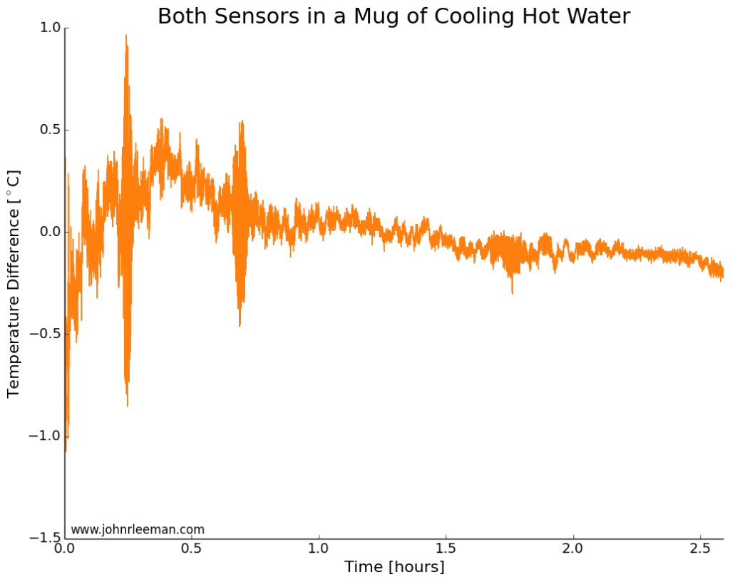
If we plot the temperature difference between the sensors it should be constant since they are sensing the same thing.  These probes look to be about dead on after calibration.  Other than the noisy segment of data, they are always within 0.5 degrees of each other.  Now we can move on to the freezer test.

CoolingWater_TempDifference

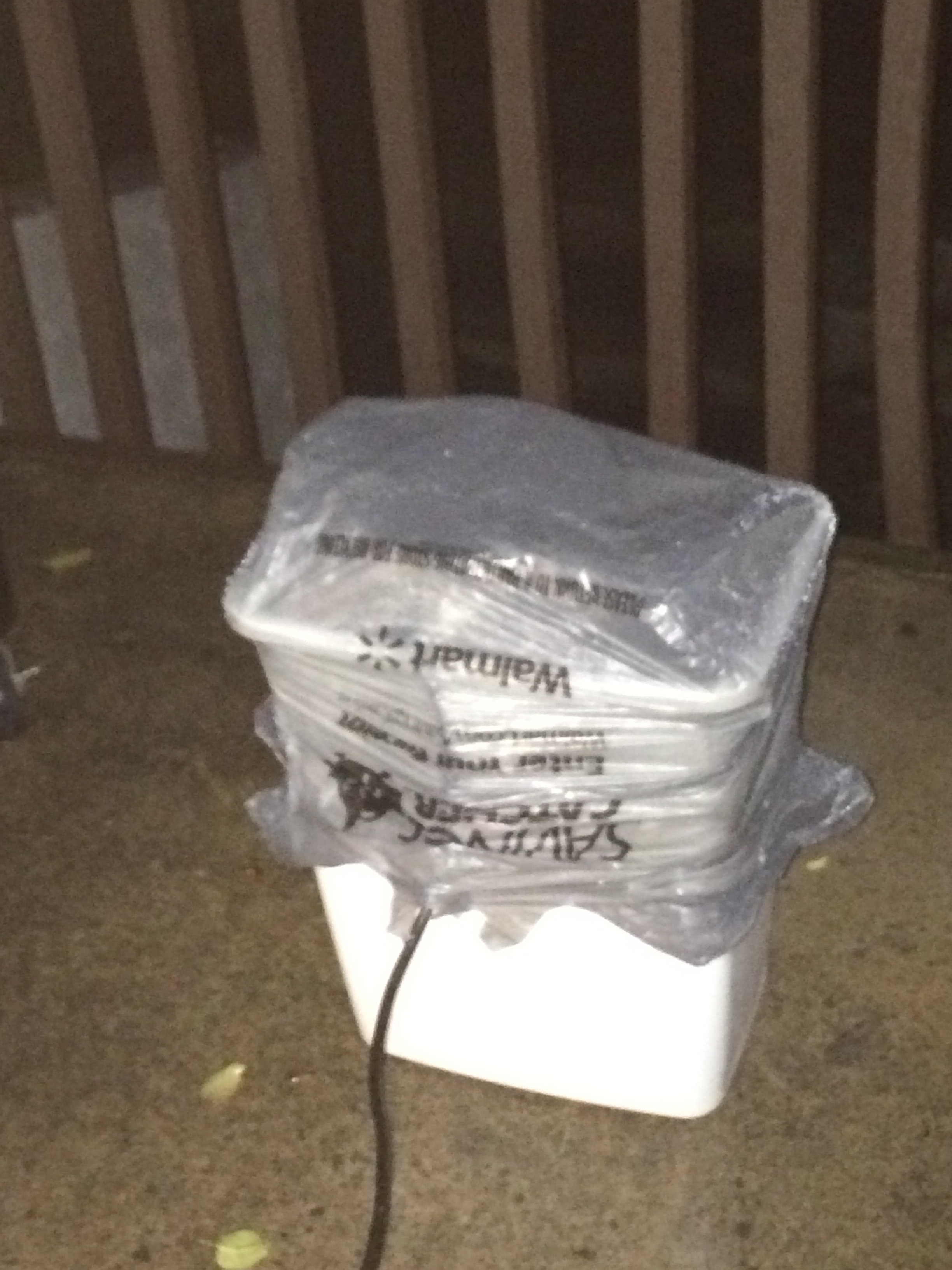
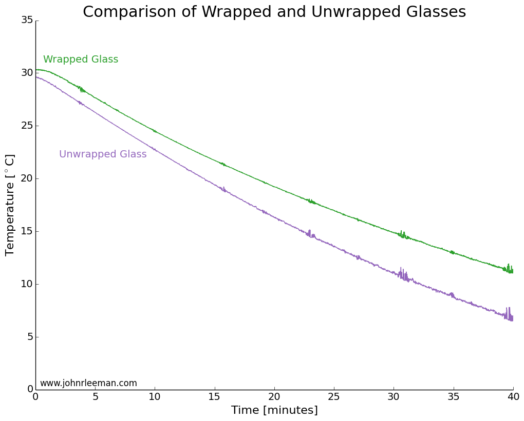
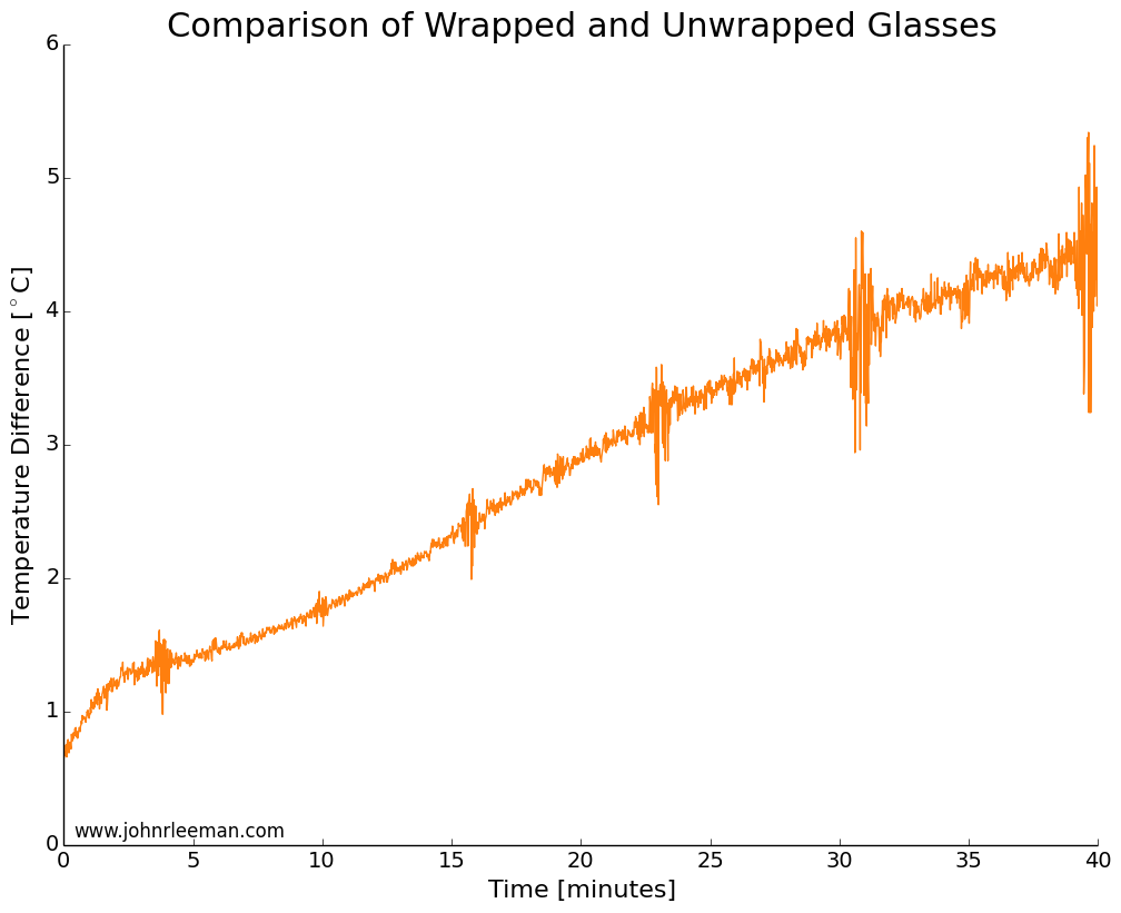
I used two identical pint glasses and made thermocouple supports with cardboard.  One glass was wrapped in tap water damped paper towel, the other left as a control.  Both were inserted into the freezer at the same time and the temperature monitored.  The water was initially the same temperature, but the readings quickly diverged.  The noisy data segments reappear at fixed intervals suggesting that the freezer was turning on and off.  The temperature difference between the sensors grew very quickly, meaning that the wrapped glass was cooling more slowly than the unwrapped glass.  This is the opposite of the myth! 

FreezingWater_AbsoluteTemps


FreezingWater_TempDifference

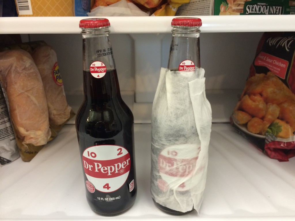
Next I placed two identical, room temperature bottles of soda in the freezer, again with one wrapped and one as a control.  After 30 minutes in the freezer, the results showed that the bottles and their contents were practically identical in temperature.  The wrapped bottle was slightly warmer, but it was within the resolution of the instruments (thermocouple and IR sensor).  I did this test multiple times and always got temperatures within 1 degree of each other, but not consistently favoring one bottle.

So what's happening here? Well, I think that the damp paper towel is actually acting as a jacket for the beverage.  Much like covering yourself when it's cold outside, the damp paper towel must be cooled, then the beverage can cool.  Adding that extra thermal mass and extra layer for the heat to diffuse through.  To provide another test of that hypothesis I again tested bottles with a control and a foam drink cooler around the base.  The foam cooler did indeed slow the cooling, the bottle being several degrees warmer than the control.

2014-08-13 17.56.28

The last question is why did the test with the glasses show such a pronounced difference, but the bottle test show no difference? My best guess is that the pint glass was totally wrapped vertically and that bottle had the neck exposed still.  Another difference could be the thickness of the towel layer and the water content of the towels.  

The Conclusion: BUSTED! Depending on how you wrap the paper towel it will either have no effect or slow down the cooling of your favorite drink.  

Let me know any other myths I should test! You can also keep up to date with projects and future posts by following me on twitter (@geo_leeman).

Arduino Code:

// which analog pin to connect
#define THERMISTOR1PIN A0
#define THERMISTOR2PIN A1
// resistance at 25 degrees C
#define THERMISTORNOMINAL 10000
// temp. for nominal resistance (almost always 25 C)
#define TEMPERATURENOMINAL 25
// how many samples to take and average, more takes longer
// but is more 'smooth'
#define NUMSAMPLES 15
// The beta coefficient of the thermistor (usually 3000-4000)
#define BCOEFFICIENT 3950
// the value of the 'other' resistor
#define SERIESRESISTOR1 9760
#define SERIESRESISTOR2 9790

int samples1[NUMSAMPLES];
int samples2[NUMSAMPLES];

void setup(void) {
Serial.begin(9600);
analogReference(EXTERNAL);
}

void loop(void) {
uint8_t i;
float average1;
float average2;

// take N samples in a row, with a slight delay
for (i=0; i< NUMSAMPLES; i++) {
samples1[i] = analogRead(THERMISTOR1PIN);
samples2[i] = analogRead(THERMISTOR2PIN);
delay(10);
}

// average all the samples out
average1 = 0;
average2 = 0;
for (i=0; i< NUMSAMPLES; i++) {
average1 += samples1[i];
average2 += samples2[i];
}
average1 /= NUMSAMPLES;
average2 /= NUMSAMPLES;

//Serial.print("Average analog reading ");
//Serial.println(average);

// convert the value to resistance
average1 = 1023 / average1 - 1;
average1 = SERIESRESISTOR1 / average1;

average2 = 1023 / average2 - 1;
average2 = SERIESRESISTOR2 / average2;
//Serial.print("Thermistor resistance ");
Serial.print(average1);
Serial.print(',');
Serial.print(average2);
Serial.print(',');

float steinhart;
steinhart = average1 / THERMISTORNOMINAL; // (R/Ro)
steinhart = log(steinhart); // ln(R/Ro)
steinhart /= BCOEFFICIENT; // 1/B * ln(R/Ro)
steinhart += 1.0 / (TEMPERATURENOMINAL + 273.15); // + (1/To)
steinhart = 1.0 / steinhart; // Invert
steinhart -= 273.15; // convert to C

Serial.print(steinhart);
Serial.print(',');

steinhart = average2 / THERMISTORNOMINAL; // (R/Ro)
steinhart = log(steinhart); // ln(R/Ro)
steinhart /= BCOEFFICIENT; // 1/B * ln(R/Ro)
steinhart += 1.0 / (TEMPERATURENOMINAL + 273.15); // + (1/To)
steinhart = 1.0 / steinhart; // Invert
steinhart -= 273.15; // convert to C(steinhart);

Serial.println(steinhart);
//Serial.println(" *C");

delay(1000);
}