Category Archives: Space

315 Million Miles From Home, Cold, and Landing on a Ball of Ice

Rosetta's_Philae_touchdown

Image: Wikimedia

Tomorrow (November 12, 2014), the Philae robotic lander will detach from the parent spacecraft, Rosetta, and begin its short trip to the surface of comet 67P/Churyumov–Gerasimenko. This is a big step in technology and spaceflight! I'm sure we'll hear lots of fascinating new discoveries in the coming weeks, but before the lander detaches I wanted to point out how amazing this mission already is and a few things that it has already taught us.

First, let's talk about distance and speed. Space often confounds us with mind-boggling distances, sizes, and speeds. Rosetta was launched in 2004 and made a few loops in the inner solar-system to use gravitational acceleration to help it get out past Mars. As of this writing, Rosetta was about 315 million miles away from Earth, having actually travelled much further (map below). It is orbiting a small body (a comet) that is traveling at about 44,700 miles per hour (20 km/s). It is also orbiting very low to the comet, only about 19 miles (30 km) off the surface.

Image: ESA

Image: ESA


In the morning, at about 3:35 AM Eastern Time, the Philae probe will detach from the orbiter and begin the seven hour journey to a landing on the comet's surface. Not only is landing on a moving target far from home difficult, but it is made even more difficult by the small size of the comet. We know that small bodies exert less gravitational attraction on other objects (it's directly proportional to the mass if you remember the Law of Gravitation). Small masses are normally good, because it means that we don't have to be going as fast to escape the gravitational influence of the planet. For example, the escape velocity of Earth is about 25,000 miles per hour (11.2 km/s), while the escape velocity of the moon is only about 5,400 miles per hour (2.4 km/s). The escape velocity of the comet is only about 1.1 miles per hour (0.5 m/s)! Since the spacecraft is descending at about 1 m/s, this presents a problem: it would likely touch the comet, then bounce off, never to be seen again.

To solve the landing problem, Philae has legs with a strong suspension system that utilizes the impact energy to drive ice-screws into the surface. For additional security, two harpoons will be fired into the surface as well.

One of the ice drills securing the lander. Image: Wikimedia

One of the ice drills securing the lander. Image: Wikimedia


Once on the comet, the suite of 10 instruments will begin to collect data about the magnetic field, composition, and other parameters. I'm sure the team will have many fascinating discoveries to share, but in the interest of keeping this post short, I'd like to share one result we already have.

Rosetta has been, and will continue, to collect data from orbit with radar units, cameras, magnetometers, and spectrometers. As Rosetta began to get close, scientists noticed a periodic variation in the magnetic field around the comet. These variations are very low in frequency, about 40-50 milli-Hertz. We can't hear anything that low in frequency, but if you artificially bump up the frequency so we can listen to the data, you get the following:

What is most fascinating about this is that it was totally unexpected! Scientists are unsure of the cause. This is one of the many puzzles that Rosetta and Philae will reveal, along with a few of the answers. Best of luck to the team. We'll check in on the spacecraft again in the future and see what we've learned.

One last note: even traveling at the speed of light, the radio signal confirming the spacecraft status will take about 30 minutes to travel from Philae to us! Be sure to watch live tomorrow (here).


Gravitational Tricks: Lagrange Points and Orbiting at Puzzling Speeds

The orbital path of ISEE3 from launch to near present.

The orbital path of ISEE3 from launch to near present.

Last time I talked about a team trying to capture and reuse the ISEE3 satellite (here).  The team has received lots of telemetry lately, determined the rotation speed of the satellite, and even had an amateur radio operator receive the satellite!  While all of this is going on, they must rapidly plan out what orbit they wish to enter.  The most discussed orbit is termed ESL1, the Earth-Sun system Lagrangian point #1.  Lagrange points an interesting phenomena that I thought worth a short discussion.

When we think of orbits, traditionally we consult Kepler's laws.  These "laws" are 3 simple rules that were written down between 1609 and 1619 by Johannes Kepler.  I won't discuss them at length, because there are already many great sources to learn about Kepler's Laws and their application.  The thing we want to draw from them is that an object orbiting closer to the Sun (say Venus), will have to travel faster to satisfy the laws of nature.  In doing so it will orbit the Sun more times than the Earth will in the same amount of time.  Venus will in fact orbit the sun 1.6 times during 1 orbit of the Earth!

Let's say we place a satellite far away from the Earth, between the Earth and sun.  the satellite will orbit slightly faster than the Earth.  Over a period of time it will be on the opposite side of the Sun and we won't be able to communicate.  Eventually it will come around and lap the Earth! This isn't desirable, but we can use Lagrange points to solve this problem.

The simple laws of orbital mechanics that we have considered thus far are only valid for a simple problem with two objects (Earth and Sun or Earth and Satellite).  We have we three bodies though, the Earth, the Sun, and the satellite! Three body problems are generally sticky to solve, but we have an advantage.  The mass of a satellite is small compared to the mass of the Earth and the mass of the Sun (unless it's the Death Star).   We can ignore the small mass of the satellite as solve what is known as the restricted three body problem.  There are a few interesting points in space, the Lagrange points, at which the gravitational pull from the Sun and Earth are superimposed on each other to give the satellite the same orbital speed as the Earth!

The L1 point is where ISEE3 may end up, so let's look at it.  The satellite will be above the Earth at an altitude of 1.5 million km (932,000 miles), towards the Sun.  At this point, the two body mechanics say that the satellite will orbit the Sun faster than the Earth.  Adding in the complications of the three body problem, we see that the gravitational tug of the Earth towards the Earth,  away from the Sun is canceling out just enough of the Sun's pull to make the satellite orbit at the same angular speed as the Earth.  How useful!

There are other Lagrangian points as well (L2-L5), but we won't discuss them here, other than to say that a similar explanation can be given for each.  L4 and L5 are particularly interesting because they are inherently stable and hence lots of objects get caught there.  There are objects in Earth-Sun L4/L5 and Earth-Moon L4/L5.

Lagrange Points of the Earth-Sun system (Image: Wikipedia)

Lagrange Points of the Earth-Sun system (Image: Wikipedia)

Generally satellites are placed in a small orbit around the L1 point for several reasons, including that it isn't inherently very stable.  The ISEE3 team will have to execute a rather complex series of maneuvers to get to L1 again, using the pull of the moon and making a very close pass that comes within 10's of km of the surface of the moon.  Time is of the essence, as the longer the wait the more they must change the speed of the craft (referred to as Delta V in the engineering jargon).  The ship only has about 150m/s of Delta V left before it runs out of fuel.  It'll take up to 1/3 of that to reposition the satellite, depending on how long the team must wait.

That's the quick and dirty view of Lagrangian points.  I hope this was interesting and helps you understand space exploration, or your addiction to Kerbal Space Program a little more!

Reviving a Piece of the 1970's: ISEE-3

hello.again.m

There's been a decent buzz in the space and tech communities about the "ISEE-3 Reboot Project", so I thought it would be worth mentioning here and pointing out some of wonderful techniques they are using to revive a satellite from almost 40 years ago.

The ISEE-3 satellite is one of three satellites that made up the International Cometary Explorer (ICE) program.  There were some interesting orbital things done with this satellite after its launch in August of 1978.  It was also the first spacecraft to go through the tail of a comet!  As with all missions, this one came to an end and the satellite was not head from since 1998.  The equipment to talk to the satellite was removed and it was considered to be out of service.

ISEE-3 sits in a heliocentric orbit, meaning that orbits the sun, not the Earth.  We knew that ISEE-3 would make another stop by our planet in 2014 when it was parked in this orbit in 1986 (from what I can tell anyway).  A group of citizen scientists started the ISEE-3 Reboot project, crowd funded on the internet.  They got permission to take over the satellite and intend to use the Moon's gravity and a rocket burn to send it on another mission.  If the window of June is missed, the satellite will probably never be heard from again.

The team was able to contact ISEE-3 on May 29 using the Arecibo observatory radio telescope.   The craft was commanded to transmit engineering telemetry, basically a health screening of the systems.  The team is currently busy decoding the data (streaming in at 512 bits/sec) and planning how they will execute the rocket burn.

The team is running out of an old McDonalds at the NASA Ames Research Park, the makeshift mission control has been termed "McMoons" after hosting previous space based projects.

IMG_3113


The part of this that I find amazing is the role that software defined radio is playing.  Software defined radio (SDR) is a way to use software to emulate radio equipment.  With a small USB stick I can receive many different kinds of radio signals and decode them, something that would have required racks of equipment a few years ago.  This team is using a radio termed the "USRP" that allows them to transmit and receive.  I've written about them before (here) and have used them in research.  They are amazing little units and provide a unique learning opportunity.  (Maybe I'll post something about a radar we made with one of them as a demo!)  A photo tweeted by the team shows 2 USRP units and laptops hooked into the giant dish antenna at Arecibo.

Screen Shot 2014-06-02 at 12.51.08 PM


That's all for now, but stay tuned to the team's website for updates and I'll be keeping up with the progress as well.  This is just another incredible example of how advanced hardware and software that has become relatively cheap can allow a group of savvy citizens to accomplish incredible feats!  Way to go folks!


KickSats - An Interview with Zac Manchester

Another AGU related post, but this time one that offers a future opportunity for participation! While walking around the vendors areas I approached a space company and began talking with a student at their booth. He turned out to be Zac Manchester, the main driver of the KickSat campaign. We chatted for a bit and I thought this would make a great post as well as letting you know about an upcoming opportunity to help telemeter data down.

Zac Manchester showing off an example satellite at the AGU Fall Meeting.

Zac Manchester showing off an example satellite at the AGU Fall Meeting.

You can find out some about the project from KickSat.net. After the meeting Zac was kind enough to answer some questions for the blog. There will be a future post as well where I'll share my personal ground station setup and then posts during reception of the data in Feburary. It's fun to see these tiny satellites that are just a printed circuit board with a solar cell and no battery. Amazing design and great use of a Texas Instruments microchip with a built in radio! Zac actually repurposed these chips as they are designed to be used in wireless key entry systems in cars. Fantastic!

What inspired you to start the KickSat program?
Mostly desperation. Our research group at Cornell has been working on
"ChipSat" scale spacecraft for a number of years and we got to a point
where we felt we were ready to actually fly some in space. We were
able to get a free launch through a NASA program called ELaNa, but we
still needed some money to build the flight hardware. KickStarter was
still pretty new at the time (2011), but I had heard of it through
some friends. After thinking it over a lot and not really having many
other options, we decided to go for it.

What was the most difficult challenge during the project?
The most difficult technical challenge was probably the communications
system. We're trying to simultaneously receive signals from over 100
tiny satellites, each with only about 10 mW of power, from 500 km
away, all on a very low budget.

How will the satellites be deployed and where can we find tracking data?
The Sprites will be deployed out of a 3U CubeSat "mothership" (called
KickSat), which is being launched on a SpaceX Falcon 9 in late
February or early March. The Sprites will be deployed 7 days after
launch vehicle separation and we will have tracking data available on
our website (kicksat.net).

When is launch?
Officially February 22, 2014, but that will likely be subject to delays. This is now set for March 16, 2014.  You can check for updates by looking for spacecraft "SpaceX CRS 3" on  SpaceFlight Now.

How long will the satellites be in orbit?
KickSat, the 3U CubeSat "mothership" will stay in orbit for a few
months, while the Sprites will reenter in a few days, probably less
than a week, after they are deployed.

How can educators and radio operators receive the data? How should be send in any data we receive?
We'd love to have participation from as many radio amateurs as
possible. Information on how to set up a ground station, receive
signals, and submit recorded data will be posted on kicksat.net in the
coming weeks.

That's it! Thank you for reading and be sure to check out any follow up posts.  I'll be setting up my ground station over the next week.

Remembering Challenger: 28 Years

722342main_challenger_full_full

It's been 28 years since the Space Shuttle Challenger (STS-51-L) broke apart just over a minute after launch.  Disasters like Challenger and Columbia remind us that space exploration really is a complicated and risky business.  Should we stop because something is risky? Absolutely not, but we should also not let such things become routine and fall out of the public view.

Remembering the Challenger Crew

The NASA family lost seven of its own on the morning of Jan. 28, 1986, when a booster engine failed, causing the Shuttle Challenger to break apart just 73 seconds after launch.

In this photo from Jan. 9, 1986, the Challenger crew takes a break during countdown training at NASA's Kennedy Space Center. Left to right are Teacher-in-Space payload specialist Sharon Christa McAuliffe; payload specialist Gregory Jarvis; and astronauts Judith A. Resnik, mission specialist; Francis R. (Dick) Scobee, mission commander; Ronald E. McNair, mission specialist; Mike J. Smith, pilot; and Ellison S. Onizuka, mission specialist.

Via NASA

Earthrise - 45 Years Ago Today

Earthrise Photograph

The famous "Earthrise" photograph.

On December 24, 1968 one of the most powerful photographs of our time was captured. Today being the 45th anniversary of this event, I thought a brief look back would be fitting. The crew of Apollo 8 (Borman, Anders, and Lovell) were just finishing their fourth lunar orbit when they saw an awe inspiring sight. Due to a roll maneuver being executed by the spacecraft, the Earth came into view out of the window. As the astronauts were just coming around from the far-side, the Earth was rising over the lunar terrain! This was a sight that nobody had seen before. There was a scramble for film, first a black and white photograph, then finally a color photograph as the capsule rotated further and the event came into view of another window. Listening to the crew conversation is very interesting as they hurry to photograph the event with their Hasselblad 500EL. The "Earthrise photo" is more officially known as NASA photo AS8-14-2383.

The scientific visualizations team from NASA have done a fantastic job putting together a short video showing the events that transpired with syncronized crew voice recordings. By using photos from the recent Lunar Reconnisance Orbited (LRO) and a timed camera on Apollo 8 they have even determined the exact orientation of the spacecraft during these events. I highly recommend watching it! This greatly reminds us of the sentiment Eugene Cernan expressed later in the program: "We went to explore the moon, and in fact discovered the Earth."

Seismic Evidence From the Russian Meteorite Explosion

Today we're going to follow up on the last blog post about the explosion of a meteorite over Chelyabinsk, Russia.  The process of figuring out precise infrasound arrival times is quite a tricky process, the travel times depend on winds, humidity, and many other atmospheric variables that are hard to constrain over such a long travel path.  I've had several fantastic discussions with Dr. Charles Ammon here at Penn State to try to obtain the infrasound data that was collected near the blast, but so far we have not been able to get it.  When/if we do, expect another posting.

The focus of this post will actually be the seismic data near the blast.  There are many seismometers all over the Earth that record the motion of the ground many times a second.  After some discussion of the infrasound and seismic data available with Dr. Ammon, we found some really nice, simple results that would make a great laboratory assignment for an introductory seismology or geoscience class.  The activity could range from reading times of arrivals on provided graphs for a non-majors class, to filtering and grid searching to estimate the precise detonation location for a more advanced class.  I've provided the data and some thoughts on it below.

We'll consider data from five seismic observatories, the station names are ARU, BRVK, KURK, OBN, and ABKAR.  Below is a map showing the station location, distance to the blast (red star), and a seismogram from that station.  The seismogram shows how the ground is moving through time, in this case I'm showing the "Z" component.   This really just means we're looking at how the ground is moving up and down, though these stations also record North/South and East/West movement.  What we see is ground motion caused by the shock wave hitting the ground and that ground motion propagating away.

Fig. 1 - Map view of the seismic stations used.  Distance from the explosion, time after the explosion to a phase arrival, and arrival order (rank) are shown along with the seismogram.  All seismograms begin at the instant of the explosion.

It's common sense to expect the energy from the explosion to arrive at a later time at stations further away, which it does.  Notice how the sharp peak corresponds to distance? We can actually make a plot of this and learn some more from the data.  To do this, pick a feature that is easily identified in each waveform (we used the first trough) and record how many seconds after the blast it arrives at the instrument.  We then plot that on the x-axis of a graph and the distance of the station from the blast on the y-axis.  The result should be something like that shown in figure 2.  Now we can use some basic math to figure out how fast this energy was traveling.  The red line on the figure is the "best fit line" to the data.  We use some basic statistics (a linear regression) to make this line, but any plotting program will do it for you.  A line has a slope (how steep it is) and a y-intercept (where it touches the y-axis when x is zero).  The slope of a line is how much the y values change per a certain change on the x axis, often taught as "rise over run" in the classroom.  The slope of this line turns out to be about 3km/s.  That's a pretty reasonable speed for surface waves (which these are) through the ground!

Fig. 2 - The distance from the blast against arrival times.  This data indicates the surface waves traveled about 3km/s, a reasonable speed.

If we could pick out a "p-wave" in the data (difficult for reasons we will discuss), the intercept of the line would be the height above the ground that the blast happened.  I haven't seen a really good estimate of the height, probably because the p-wave is hard to find and the speed of the meteorite. The meteorite was traveling about 40,000 mph when it exploded.  It's hard to imagine something moving that fast, so let's change around the units: that's something like 11 miles every second!

The p-wave could be hard to see because 1) it's going to be relatively small, and 2) there are waves from an earthquake in Tonga arriving about the same time as the meteorite explosion.  We know the waves we picked aren't from the tonga event, those would have arrived at all the stations at almost the same time because they were reflecting off the Earth's core.  It would be an interesting project to play with trying to pick p-waves and/or estimate their arrival window by guessing the height of detonation.

We don't have to stop here though.  This morning I saw this youtube video, a compilation of people recording the shockwave.  The meteorite had streaked past, exploded, and they were recording this when the shock wave hit.  Shockwaves behave in a funny way, but luckily it's been studied a lot by the government.  Why? Nuclear weapons! Seismologists are commonly employed to determine if a nuclear test has taken place, and estimate it's size, location, etc.  A lot of very interesting information on air-blast and it's interaction with buildings can be found in the book "The Effects of Nuclear Weapons".  The book has lots of formulas and relations that could make many interesting lab exercises, but we'll just discuss reflection in this post.

A shock wave is really a front of very high air pressure that is propagating through some material.  The high pressure is followed (in a developed shock wave) by a small, longer, suction, then a small overpressure.    I've tried to locate meteorological observations and so far have only found hourly observations.  If we can find short term observations we would expect to see wind rushing away from the blast, then more weakly towards it, then very weakly away from the blast.  By knowing those wind velocities we could estimate the pressure differential that caused the shock.  The local airport (station USCC) does report hourly average winds (data here).  There is a small bump in the average winds between 9-10am local time, when the meteorite entered.  The lack of a gust report though makes this observation a bit too shaky to use for a pressure estimate.  

Shock waves move faster than the speed of sound if they are a high enough "overpressure", or the pressure above atmospheric.  Shock waves will reflect off the ground when they reach it, as shown in figure 3.  The overpressure in the region of "regular reflection" is much higher than the overpressure of the shock wave due to a combined stacking effect.  There can also be complicating patterns such as "Mach Reflections".  

Fig.3 - The initial pressure wave (solid lines) and the reflected shock (dashed lines).  Image from "The Effects of Nuclear Weapons"

What's interesting about all this is the audio of the clips at about 20 and 40 seconds into the YouTube video.  Notice these clips contain two bangs.  The first clip with two shocks could be reflection off the building behind the camera, the second shock follows the first very close and is very loud.  The next clip has a significant delay though.  At any height above the surface the initial reflection occurred on, there will be a delay between the initial and reflected shock.  If we knew the location of this video it would help constrain the shock location.  (After some google searching I can't locate the "Assorty" store in the footage anywhere.)

Overall with the observations of glass breaking over such a large area, we can assume the reflected pressure was probably in the area of 1psi.  This means the initial overpressure was very small at the ground.  Could you work backwards from the estimate of 500 kiltons TNT? Sure! That's a topic for another day or for your students in lab! Be sure to check out the book "The Effects of Nuclear Weapons", many campus libraries have it, Penn State has it online even.

Below is a link to a zip file that contains the .SAC files for the seismic stations (starting at detonation time and low pass filtered as well as raw data) and high quality figures.  If I end up writing up a lab from the event, expect the data and lab to be on my academic website.  A review of literature on the Tunguska event may be helpful as well!

Zip file of data.

Chelyabinsk Meteorite - Infrasound, Seismic, and Satellites oh my!

Just as Earth was about to have a close encounter with asteroid 2012 DA14, the people of Chelyabinsk, Russia had a personal experience.  Before we talk about both 2012 DA14 and the Chelyabinsk event some terminology needs to be set out.  A meteoroid is a small chunk of debris in space, generally anything from a fleck of dust to a small boulder.  A larger space bit of debris is termed an asteroid.  A meteor is when some of this debris enters our atmosphere, heating up due to friction.  A meteor is called a meteorite if it actually reaches the surface of the Earth and survives impact.  Everyday we are pelted with many tiny meteors, but few reach the surface.  Most meteorites are never discovered as they are statistically much more likely to land in the ocean due to it's coverage of Earth's surface.  Sometimes meteorites are found on land, in fact it is common for scientists to go to Antarctica to look for the dark rocks on the surface of a white sheet of ice.  There are many pages on hunting meteorites  and a book as well, it's worth reading about if your curious how we find rocks that landed a long time ago.

It's worth saying that there are different kinds of space debris, some more stony, some made of almost solid metal, and some of ice.  While it's worth discussing, I'd rather focus on the current events in this post, so if you are curious there is a nice page at geology.com that gives the basics.

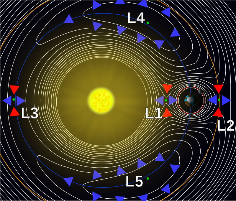
To begin, lets talk about 2012 DA14, or the non-intuitive name that we gave a near Earth asteroid that is about 160 feet in diameter and weighs a massive 190,000 metric tons.  This asteroid could do some serious damage and was scheduled to have a close call with Earth on February 15th.  How close? Well, it would be about 17,200 miles from the surface, which seems like a long way.  It's not.  The moon is 250,000 miles away (roughly) and we've been there and back in a matter of a few days.  In fact, the geosynchronous satellites that beam TV and weather data down to Earth orbit about 22,236 miles above the surface to rotate at the same rate the Earth does.  As shown in the figure below, 2012 DA14 passed between us and the geostationary satellite band; a very close call.

Why talk about 2012 DA14 in a post about a meteor over Russia? To say they are not related in any way.  They approached from entirely different directions and it just happened to be a coincidence of space and time.

Now for the event in Russia.  At 3:20:26 UTC on Feburary 15th a large meteor about the size of a schoolbus entered the atmosphere.  The 49-55 foot estimated diameter object probably weighed about 7000-10000 tons.  While heating up upon atmospheric entry the meteor "detonated" or exploded in mid-air.  This has happened before, a list of historic airbursts can be found here.  The most famous being a large explosion (also over Russia) in 1908 called the Tunguska event.  That explosion released the energy of 10-15 million tons of TNT, leveling forests and destroying an area of about 830 square miles.  The event that just occurred was about 500 kilotons of TNT equivalent, or roughly 20 times smaller.  Shock waves from the event still managed to send around 1500 people to local hospitals with shards of glass and building materials in their faces/skin from rushing to a window too see what was happening.  Videos of the entry are all over the web, in several you can hear the detonation and shock wave.

So how do we know so much about this object considering we didn't know anything about it until it exploded overhead? Well, remote sensing helps us.  When a meteor entered over Wisconsin in 2010, I wrote about following the trail on the US Doppler Radar Network (here).  This time we could see the meteor from weather satellites (Meteosat 10 image below) as well as on seismic and infrasound stations.  Another meteosat also captured several frames that have been made into a video here.  Current estimates of the entry speed are in the area of 40,000 mph with a very shallow entry angle.

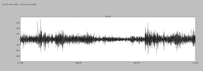
First the seismic observations.  So far I've seen reports of the Borovoye, Kazakhstan station seeing a gorgeous signal (thanks to Luke Zoet on this one). The station details, and even a photo are available at the USGS network operations page.  Below is a filtered (0.15 Hz low-pass) seismogram from BRVK.  This would be a result of the shock wave rattling the ground and seismic station.

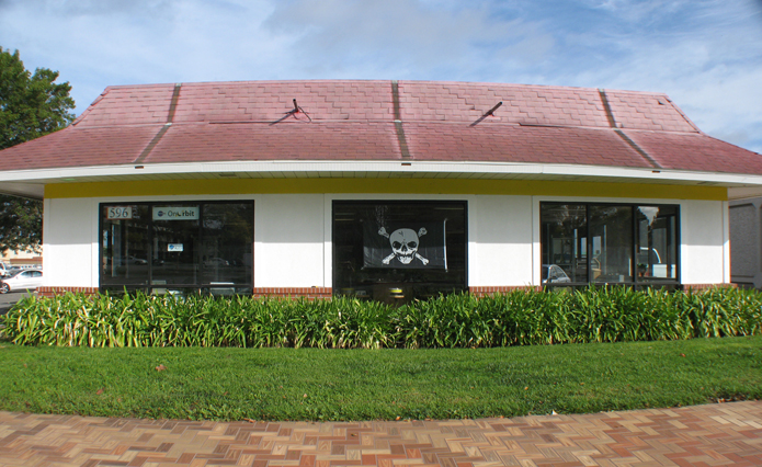
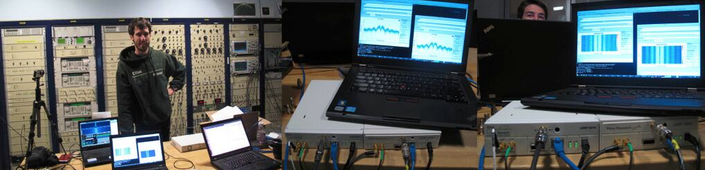
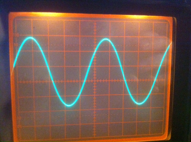
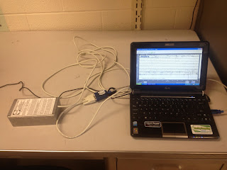
Next, and rather interesting, are the infrasound observations.  Infrasound is very low frequency sound (below 20Hz) that we can't hear, but can record as air pressure variations.  It so happens that Steve Piltz of the Tulsa National Weather Service has a microbarograph.  Upon seeing his data from an earlier earthquake (yes, ground movement causes air pressure waves), I immediately bought a unit from Infiltec and set it up in the office at Penn State.  Below is a picture of the station.

Infrasound propagation is incredibly complex and difficult to predict over such long distances, so I've done a simple calculation that is very likely going to be revised upon some discussions with seismologists this week.  First, I wanted to know how long the sound would have to travel.  To find the shortest travel distance between a latitude and longitude set you can assume a spherical Earth (not too bad for such a back of the envelope calculation) and some math.  Remember trigonometry? Well when it's modified to work on a sphere instead of in a plane it's creatively called 'spherical trigonometry' and consists of a strange function called the haversin.  If you are curious about how I calculated the travel path of the sound waves checkout the wikipedia page on the Haversine formula, but I've included the formula below.  Below is the result of the calculation, a great circle path between Chelyabinsk and State College, PA.
d = 2 r \arcsin\left(\sqrt{\operatorname{haversin}(\phi_2 - \phi_1) + \cos(\phi_1) \cos(\phi_2)\operatorname{haversin}(\lambda_2-\lambda_1)}\right)

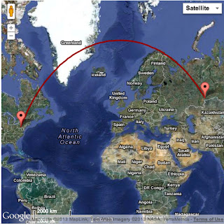
The distance the wave would travel would be something like 8670 kilometers.  Sound travels at 340.29 m/s at sea level, but since we're making assumptions we'll say 300 m/s is a nice number.  So the wave would take somewhere in the 7-8 hour range to reach State College (assuming it's non-dispersive and many other likely not so great assumptions).  Luckily for us, the event and the arrivals are overnight.  During the day my infrasound station is swamped by signals from office doors opening and closing amongst other things.  The meteor entered the atmosphere at 10:20 pm local time, so I've plotted the infrasound from 10 minutes before the meteor entered to well after the energy should arrive.  There is a large increase in the noise shortly after entry, but this is too soon.  Could it be seismic energy or arrival of a faster shock path? Maybe, that's a point for some discussion and revision later.  The big thing to notice is the noise increase at about 7-8 hours after the entry.  It's still early in the morning, so it is doubtful that this is people coming into work.

I've made a .SAC (seismic analysis code) file of the raw data for about 24 hours around the event available to download here.  Download the file (~19Mb) and play with it! The data is collected at 50Hz, but all that is in the meta-data (as well as location details).  I use ObsPy to do most of my analysis in Python, but you could use SAC or other codes meant for seismic event analysis.

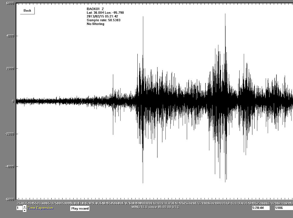
Steve's station in Oklahoma recorded similar signatures.  His data over a slightly shorter time span (5:21-11:42 UTC) is below, showing similar signatures.

Infrasound is actually what allows us to determine the energy release from the explosion.  As it turns out seismic stations and infrasound have been used to monitor nuclear testing for years (a relevant topic currently considering the recent tests by North Korea).

Overall, I'd say stay tuned for any updates.  Eventually the infrasound station I have will be setup for live streaming.  I'm sure after discussion with some folks more versed in infrasound travel we can clean up the data and maybe do some more back of the envelope energy/rate calculations for demonstation purposes.

Teaching Field Camp - Starry Nights

The geophysics students have given their final presentations and gone home.  I'll be finishing up a couple of posts (mostly waiting on graphics) about their last weeks of work and a few interesting study areas, but for now we will break from geology.  The geologists will be doing geophysics for the next few days (hence I'll still be in Cañon City), but now I'll have slightly more free time to do some photo experiments!

Saturday night another TA rushed in to tell me that the milky way was out and nicely visible.  I grabbed my camera, but sadly the moon was rising and it was hard to get great shots.  The wind was gusty, but a moon shot turned out okay, and we staged a photo with the dining hall, OU vans, and star trails.  Look for more geology posts in the next few days before I depart for my desert loop on the way to Arkansas.

Building a Fluxgate Magnetometer - Part 1 (and NASA)

Today I want to discuss the first steps in building a simple fluxgate magnetometer for a classroom demonstrator.  Originally this post was going to be a wrap up of NASA work and the magnetometer would come later, but I'm still waiting on my presentation to clear export control so I can post it.  As soon as it does, I'll put it up along with a short article.

This semester I'll be the TA for 'Global Geophysics', mostly doing lab instruction/writing.  After some thought I decided that students need more hands-on classroom geophysics, which is difficult to do.  By its nature geophysics is an outdoor activity with normally expensive instruments.  The instruments are often viewed as a mysterious black box that spits out numbers used to make a map.  This must change.  With a proper understanding of the instruments students will better understand errors in the data, how to troubleshoot in the field, and know why certain hardware limits exist.

The concept of a fluxgate magnetometer is pretty simple.  Rather than go into detail I'll refer you to this wikipedia article.  This is mainly to chronicle the construction so others can reproduce this (assuming we get a working model).  My design came from a physics lab at Brown University.  The instructions were vague in parts and I'll be taking some liberties as we go along.  This first article will cover construction of the coil and the driver circuit.

The fluxgate coil consists of a driver coil surrounding a soft steel wire, and a secondary coil to pickup signal surrounding the primary coil.  First I took 16ga annealed steel wire from Lowes and cut it to about 1m long, cleaned it, and made it as straight as possible.  Afterwards I wrapped close to 2000 turns of 22ga magnet wire (Radio Shack #278-1345) tightly along its length.  This was then bent in half making a 'U' and that was wrapped with close to 1000 turns of 26ga magnet wire. I used large wire because it will be more durable and I used different gauge wire since the enamel insulation was a different color allowing students to easily see the windings.

That's all there is to the coil.  To increase durability I will probably clear coat the coil and place it into a small acrylic tube so its difficult to bend or break.  The next step is to build a driver for the primary coil.  The Brown lab used a function generator.  Currently I don't have one, nor have I found a suitable cheap unit.  This meant improvising, and luckily Velleman makes a signal generator kit that is just about right.  It operates at 1kHz (the desired frequency for this project) and produces sine, square, triangle, and integrator waves.  The kit was pretty easy to build in just about an hour and works well as seen by the oscilloscope output below, but frequency stability is not phenomenal (especially when then unit is cold).  

Next a few amplifiers need to be designed and built.  The signal generator kit cannot pull the load of the coil, so a simple +/- 9V system will probably do.  The output will also need some kind of amplification.  The lab I found also uses a bandpass filter.  Once the amplifiers are working it will be time to decide if this is necessary and if I want to use an oscilloscope and hardware filters, or an ADC and display the waveform on a computer projector using software filters.