Going to the Science Fair

2015-02-23 19.16.17

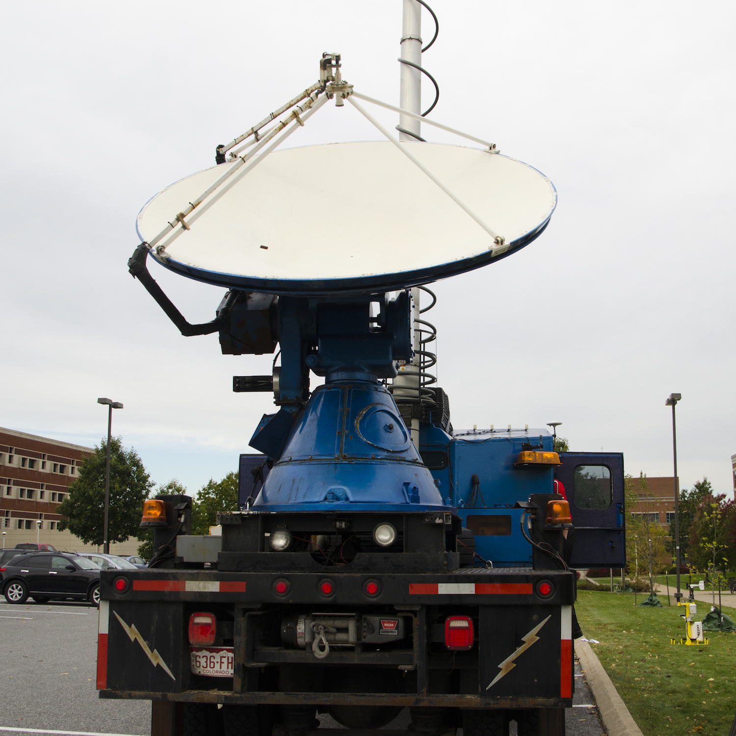
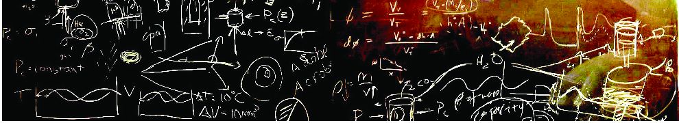
Explaining doppler RADAR with an actual demo!


This past week I got to relive some of my favorite days of primary education: the science fair!  A local elementary school was hosting their annual science fair and had asked the department to provide some demonstrations for the parents and students to see. I immediately volunteered our lab group and began to gather up the required materials. Some of the setups were made years ago by my advisor. I also developed a few and improved upon others here and there. I thought it would be fun to share the experience with you.

2015-02-23 18.09.58

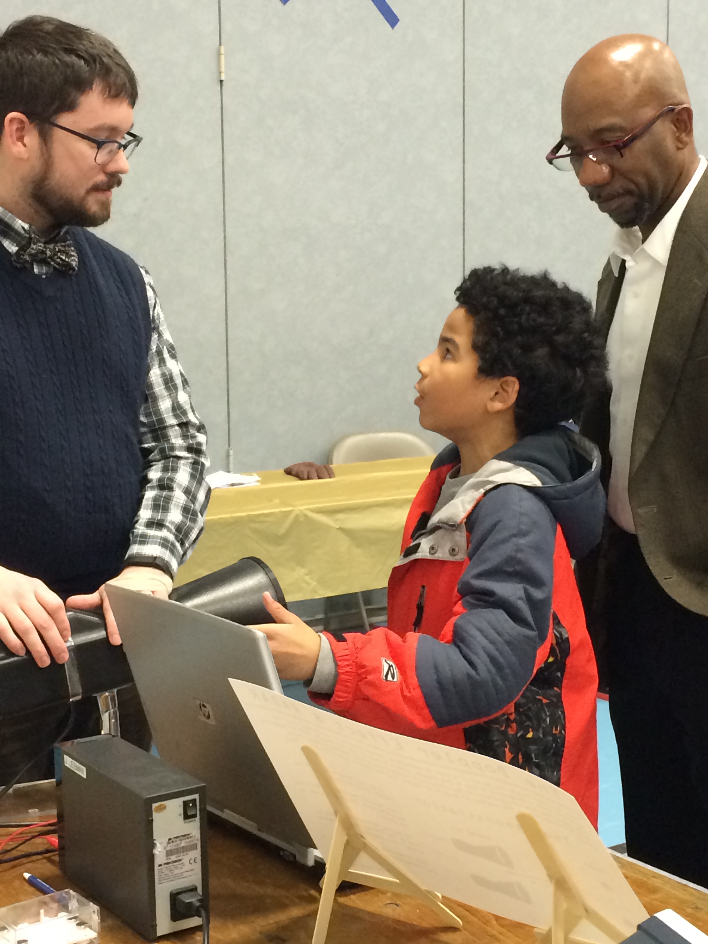
The line-up of demonstrations setup as the science fair was getting started.


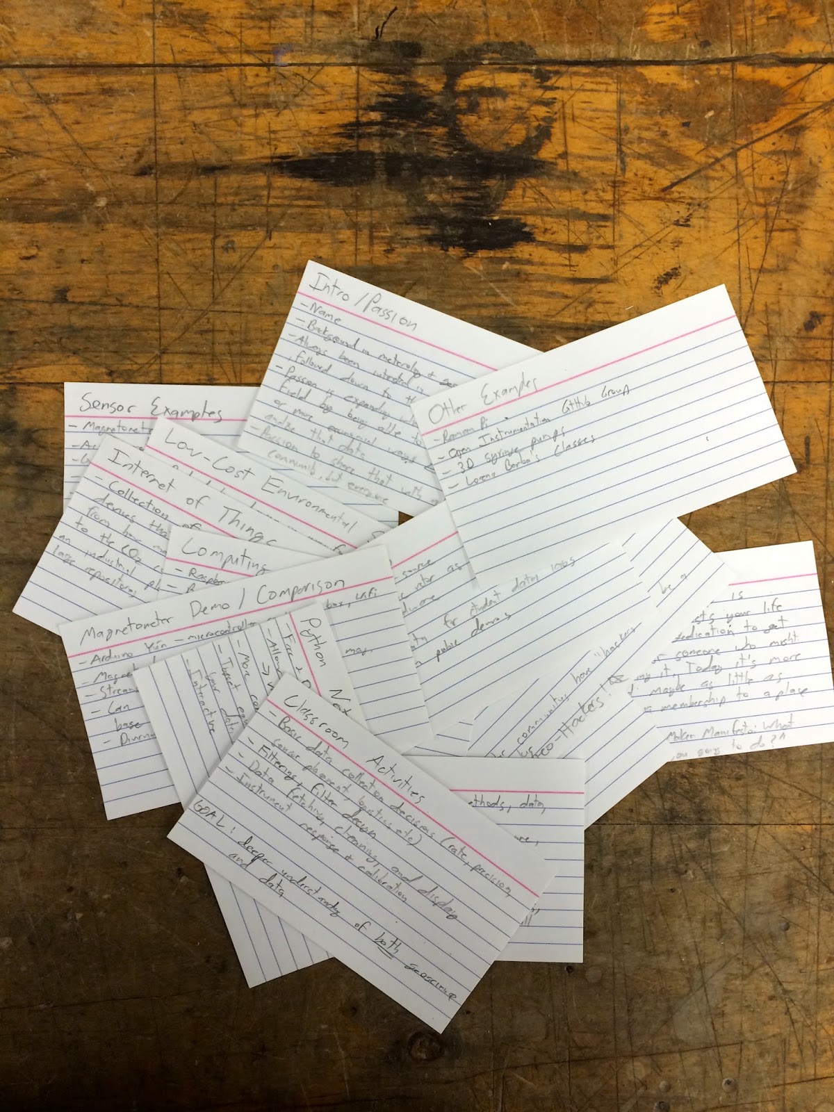
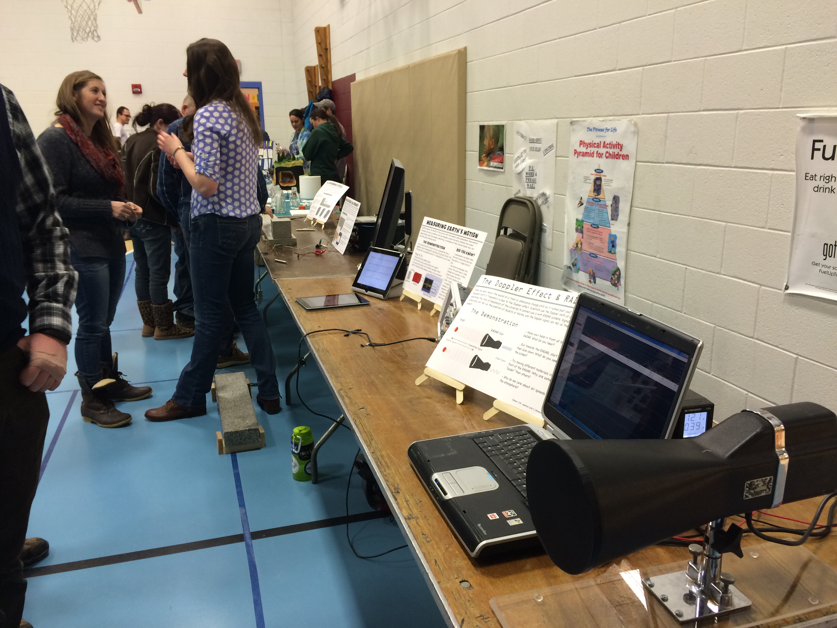
At some point, we should probably have a post or two about each of these demonstrations, but today we'll look at pictures and talk about the general feedback I received. First, off we had four demonstrations including the earthquake cycle, how rocks are like springs, seismometers, and Doppler RADAR. I made an 11x17" poster for each demo in Adobe Illustrator using a cartoon technique that one of our professors here shared with me.

Screenshot 2015-02-28 14.41.01

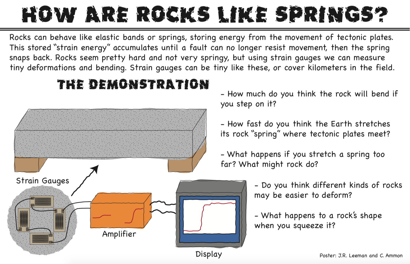
Here is an example poster from one of the demonstrations.


For scientists, communicating with the public can be difficult. It's easy for us to get holed up in our little niche of work and forget that talking about a topic like power spectra isn't everyday to pretty much everyone. Outreach events like this present a great opportunity to work on those skills! This particular event was especially challenging for me because the children were K-5, much younger than I usually talk to. With high school students you can maybe talk about the frequency of a wave and not get too many lost looks, but not with grade-schoolers!

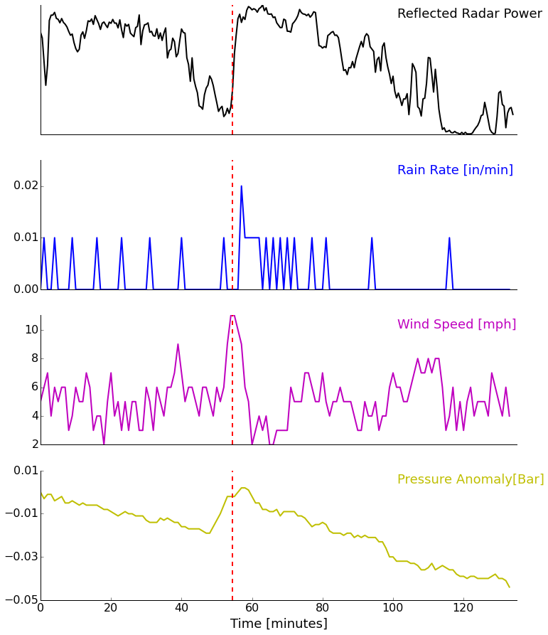
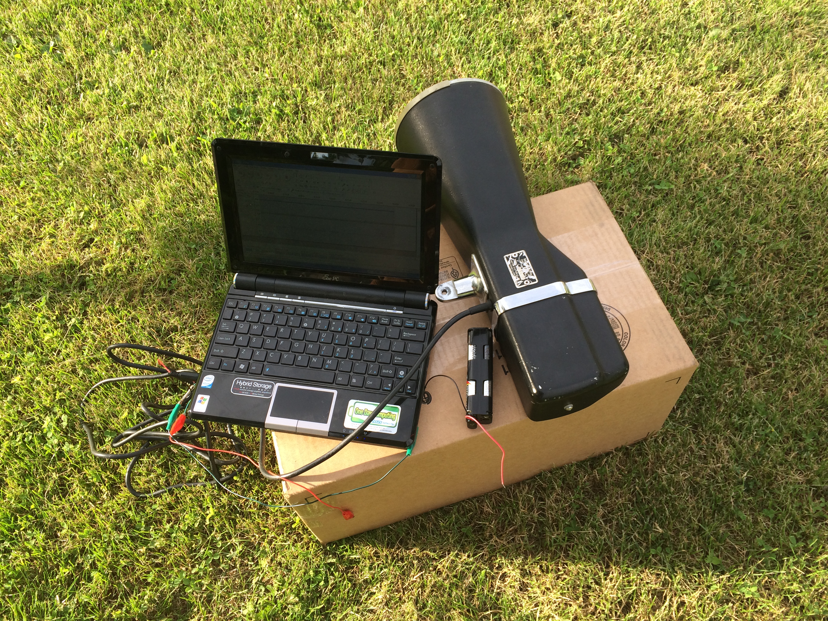
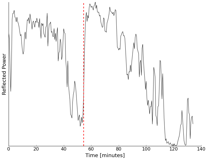
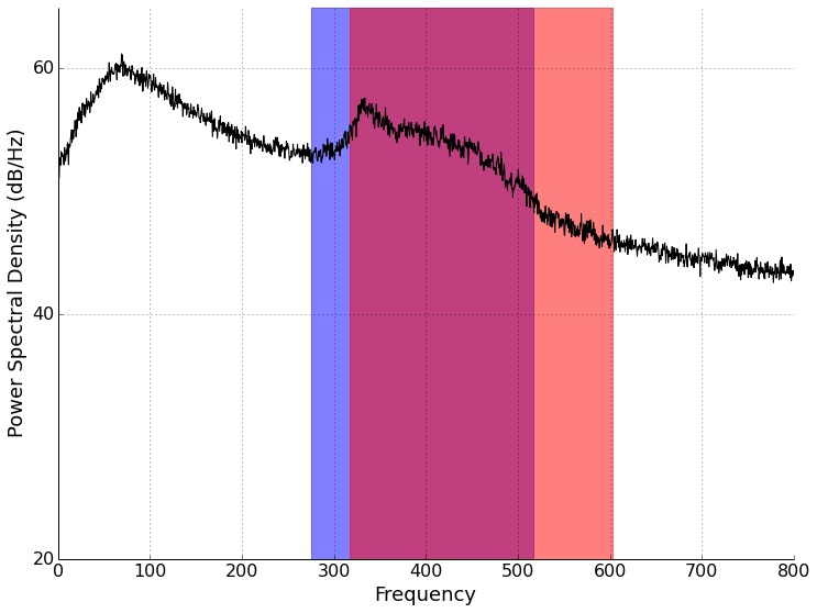
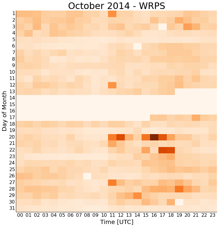
The other difficulty was adapting what are deep topics (each demo is an entire field of research, or several) to the short attention span we had to work with. Elementary school teachers are masters of this and I would love to get some ideas from them on how to work with the younger minds. I spent most of my time talking about the Doppler effect with the RADAR (it's the topic my lab mates were least comfortable with since we don't deal with RADAR at work generally). By the end of the science fair, I had an explanation down that involved asking the kids to wave their hand slowly and quickly in front of the RADAR and listen to how the pitch of the output changed. Comparing that to the classic example of the pitch bending of a passing fire truck siren seemed to work pretty well. I had a "waterfall" spectra display that showed the measured velocity with time, but other than trying to get the line to go higher than their friends, it didn't get much science across (though lots of healthy competition and physical exercise was encouraged).

2015-02-23 18.16.49

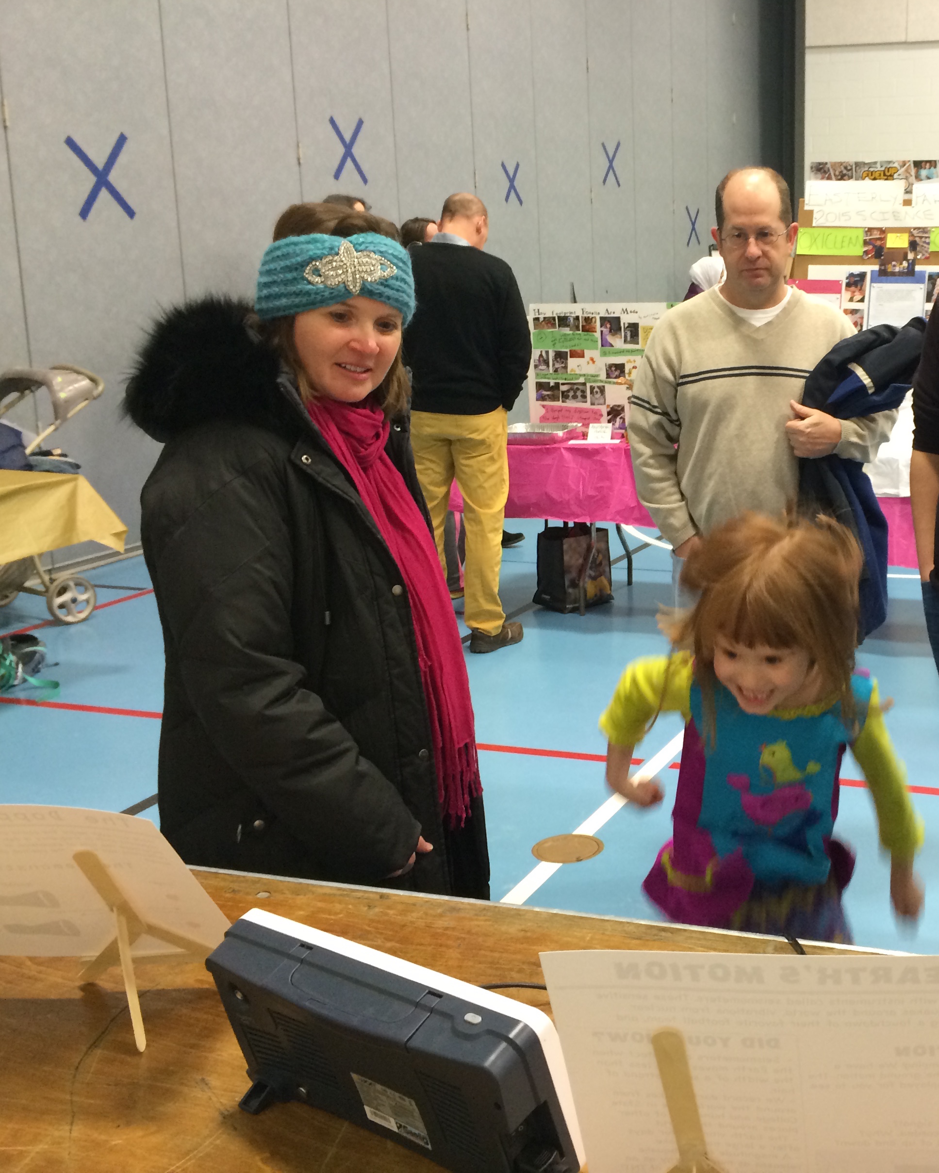
An excited student jumps up and down to see herself on a geophone display.


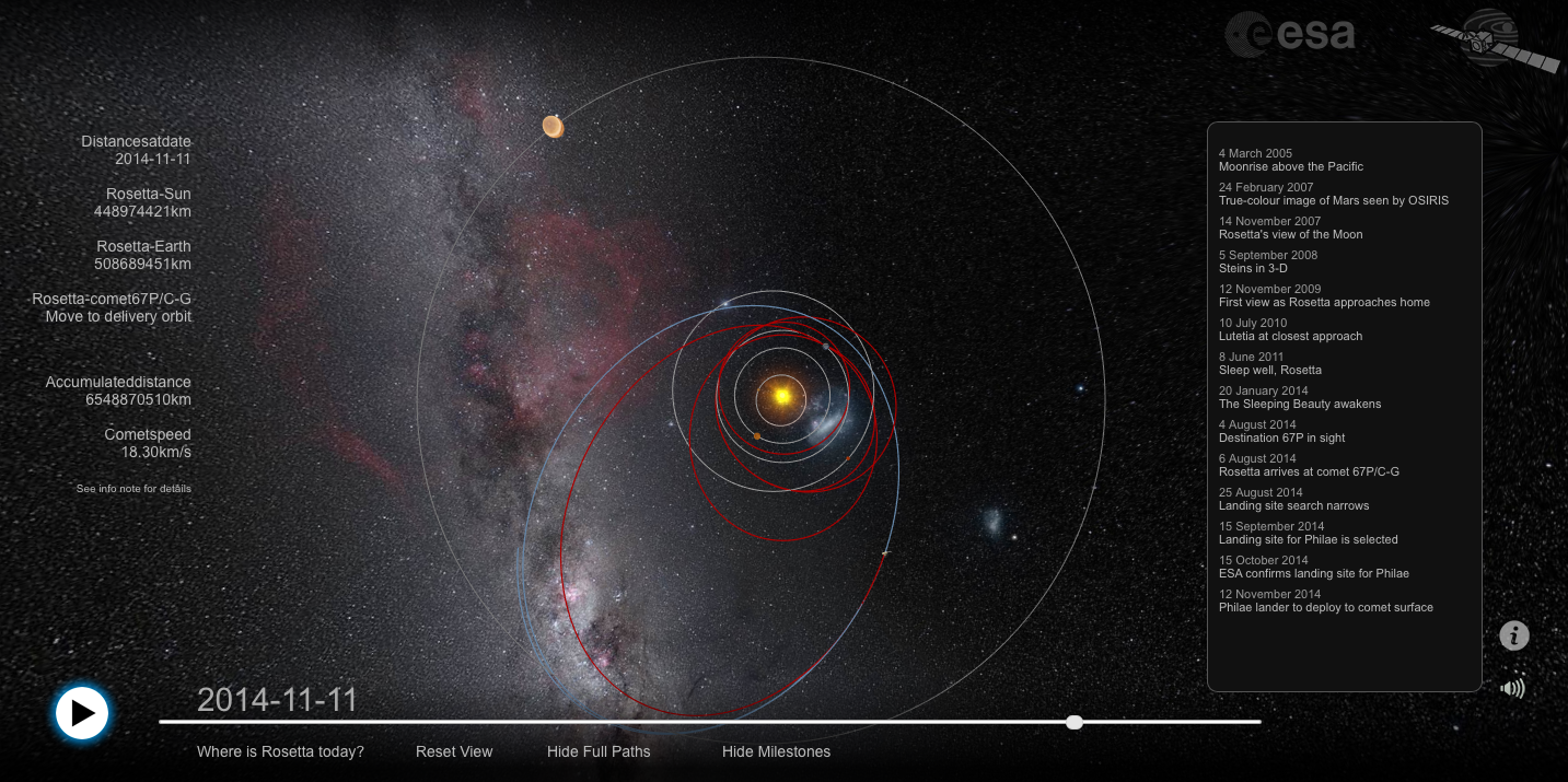
In the past, I've pointed out the value of being an "expert generalist". All of us were tested in any possible facet of science by questions from the kids and their parents. I ended up discussing gravitational sling-shot effects on space probes with a student and his parents who were incredibly interested in spaceflight. I also got quizzed about why the snow forecasts had been so bad lately, when the next big earthquake would be, and a myriad of other questions. Before talking to any public group, it's also good to make sure you are relatively up-to-date on current events, general theory, and are ready to critically think about questions that sound deceptively simple!

The last point I want to bring up today is the idea of comparisons. These are numbers that one of my committee members likes to say he "carries around in his shirt pocket." These are numbers that let us, as scientists, relate to others that are non-specialists and give us some physical attachment to a measurement.  What do I mean? Let's say that I tell you that tectonic plates move anywhere from 2-15 cm/year. Great, first, since we are in the U.S.A., everyone will hold out their fingers to try to get an idea of what this means in imperial units.... not quite 1-6 in/year. That's better, but a year is a long time and I can't really visualize moving that slowly since nothing I'm used to seeing everyday is that slow... or is it? Turns out that fingernails, on average, grow 3.6 cm/year and hair grows about 15 cm/year. Close enough! In Earth science we have lots of approximate numbers, so these tiny differences are not really that bad. Now let's revise our statement to the kids to say: "The Earth is made of big blocks of rock called plates. These move around at about the speed your finger nails or hair grow!" Now it is something that anyone can relate to, and next time they clip their nails or get a hair cut, they just might remember something about plate tectonics! It's not about having exact figures in the minds of everyone, it's about providing a hand-hold that anybody can relate to! This deserves a post to itself though.

That's all for now, but I'd love to hear back from anyone who has elementary education experience or has their own "shirt pocket numbers."


Raindrops Keep Falling on my Radar - Part 2

Last time we looked at the raindrop fall speed of raindrops during a thunderstorm and compared the radar reflected power to my observations of the storm moving through State College. Today, thanks to Yvette Richardson and Bill Syrett from the Penn State Meteorology Department, we can compare the radar returns to actual weather station data. They were able to provide data from a weather station on top of the meteorology building on campus, about 3 miles from where my radar was located.

We expect more power to be returned to the radar during periods of heavy rain, so the main variable of interest is the rain rate. We'll plot up a couple of other meteorological variables just for fun as well. The weather station recorded observations every minute. I had to venture my best guess at the units based on their values. The rain rate values are low. Another station that I don't have the time-series for reported a maximum rain rate of 0.26 in/hr. Either way, let's examine the relative changes.

rain_wx_data_graph


Looking at the plot we can see that our prediction of higher rain rate equaling more reflected power holds. Unfortunately, the weather station didn't record precipitation rate with very fine resolution, so we really can only match the peak rain rate with the peak reflected power. The vertical red line marks the time of a weather service doppler radar screenshot we looked at in the last post that was right before the heaviest rain arrived. We also observe the higher wind speeds with the gust front ahead of the storm. As the storm passed over we saw decreasing pressures as well. The temperature and humidity aren't shown because they really weren't that interesting.

Now that we've verified our hypothesis (roughly anyway) about precipitation rate and radar return, we are ready to look at different types of reflectors. Next time, we will look at radar data collected during a snow storm for return intensity and the fall speed of snow flakes. That speed can be compared with video of falling snow for verification. Stay tuned!

Raindrops Keep Falling on my Radar - Part 1

What's the most complicated way to say it's raining? Well, if you know me, you know it will involve electronics, sensors, and signal processing! This post was originally going to compare the fall velocity for rain, sleet, and snow. Unfortunately, I haven't been lucky enough to be home to run my radar when it was snowing. It will happen this winter, but we'll start looking at some data now. Want to review radar before we get started? We have already talked about looking at the doppler signature of cars and got a tour of a mobile weather radar.

Back in October we had a couple of squall lines come through. On the 3rd, there was a significant event with two lines of storms. I had just been experimenting with measuring rainfall velocity with the modified X-band radar, so I decided to try another experiment. I put the radar unit in a trashcan and covered it with plastic bags. Then I sat it outside on our balcony and recorded for about 2.5 hours.

Testing the radar setup before the rain with some passing cars as targets.

Testing the radar setup before the rain with some passing cars as targets.

There is a radar in there! My make-shift rain proof radome. The only problem was a slight heat buildup after several hours of continuous operation.

There is a radar in there! My make-shift rain proof radome. The only problem was a slight heat buildup after several hours of continuous operation.

Not only do we get the doppler shift (i.e. velocity of the raindrops), but we get the reflected power. I'm not going to worry about calibrating this, but we can confidently say that the more (or larger) raindrops that are in the field of view of the radar, the more power will be reflected back.

First, let's look at a screenshot of the local weather service radar. You can see my location (blue cross) right in front of the second line of showers. At this point we had already experienced one period of heavy rain and were about to experience another that would gradually taper off into a very light shower. This was one of the nicer systems that came through our area this fall.

A capture of our local weather radar, my location is the blue cross directly ahead of the storm.

A capture of our local weather radar, my location is the blue cross directly ahead of the storm.

Now if we look at the returned power to the radar over time, we can extract some information. First off, I grouped the data into 30-second bins, so we calculate the average returned power twice per minute. Because of some 32-bit funny business in the computations, I just took the absolute value of the signal from the radar mixer, binned it, and averaged.

Reflected power received by the radar over time. The vertical red line is the time that the radar screen shot above was taken.

Reflected power received by the radar over time. The vertical red line is the time that the radar screen shot above was taken. We can see the arrival and tapering off of the storms.

From this chart we can clearly see the two lines of storms that came over my location. We also see lots of little variations in the reflected power. To me the rain-rate seemed pretty constant. My best guess is that we are looking at skewing of the data due to wind. This could be solved with a different type of radar, which I do plan to build, but that doesn't help this situation.

Let's look at what inspired this in the first place, the rainfall velocity. From a chart of terminal velocities, we can see that we expect to get drops falling between 4.03-7.57 m/s for moderate rain and 4.64-8.83 m/s for heavy rain. Taking a 5 minute chunk of data starting at 60 minutes into the data (during high reflectivity on the chart above), we can compute the doppler frequency content of the signal. Doing so results in the plot below, with the velocity ranges above shaded.

psd_velocity

Doppler frequency content of 5-minutes of data starting at 60 minutes into recording. The blue box shows doppler frequencies corresponding to moderate rain, and the red box corresponding to heavy rain.

Based on what I see above, I'd say that we fall right in line with the 0.25"-1" rain/hour data bracket! There is also the broad peak down at just under 100 Hz. This is pretty slow (about 1 m/s). What could it be? I'm not positive, but my best guess is rain splattering and rebounding off the top of my flat radar cap. I'm open to other suggestions though. Maybe part of this could be rain falling of the eve of the building in the edge of the radar view? The intensity seems rather high though. (It was also suggested that this could be a filter or instrument response artifact. Sounds like a clear air calibration may help.)

So, what's next? We'll take some clear-air calibration data and the use data from a Penn State weather station to see what the rain rate actually was and what the winds were doing. Maybe we can get a rain-rate calibration for this radar from our data. See you then!

Thank you to Chuck Ammon for discussions on these data!


Don't Panic Geocast - Now on Your Radio!

DSCF4046

I would like to announce the official release of the first episode of the "Don't Panic Geocast!" This is something that has been in the works since earlier this summer. Each week Shannon Dulin and I will be discussing geoscience (geology, meteorology, etc) and technology. Please be sure to add us to your feeds and checkout our first show!

Sensors, Sensors Everywhere!

This year at the fall meeting of the American Geophysical Union, I presented an education abstract in addition to my normal science content. In this talk, I wanted to raise the awareness of how easy it is to work with electronics and collect geoscience relevant data. This post is here to provide anyone that was at the talk, or anyone interested, with the content, links, and resources!

Sensors and microcontrollers and coming down in price thanks to mass production and advances in process technology. This means that it is now incredibly cheap to collect both education and research grade data. Combine this with the emergence of the "Internet of Things" (IoT), and it makes an ideal setup for educators and scientists. To demonstrate this, we setup a small three-axis magnetometer to measure the Earth's magnetic field and connected it to the internet through data.sparkfun.com. I really think that involving students in the data collection process is important. Not only do they realize that instruments aren't black boxes, that errors are real, and that data is messy, but they become attached to the data. When a student collects the data themselves, they are much more likely to explore and be involved with it than if the instructor hands them a "pre-built" data set.

For more information, watch the 5-minute talk (screencast below) and checkout the links is the resources section. As always, email, comments, etc are welcome and encouraged!

Resources

Talk Relevant Links

- Slides from the talk
- This blog! I post lots of electronics/data/science projects throughout the year.
- Raspberry Pi In The Sky
- Kicksat Project
- Weather Underground PWS Network
- uRADMonitor
- Our IoT magnetometer data stream
- Python Notebooks
- GitHub repository for the 3D Compass demo
- AGU Pop-Up Session Blog

Parts Suppliers

- Adafruit
- Sparkfun
- Digikey
- Element14

Assorted Microcontrollers/Computers

- Beagle Bone
- Raspberry Pi
- Arduino
- Propeller
- MBed
- Edison
- MSP430
- Light Blue Bean

General

- Thingiverse 3D printing repository
- Maker blogs from places like Hackaday, MAKE, Adafruit, Sparkfun, etc

How I Design a Talk

This year I'm co-chairing a session at the American Geophysical Union meeting called "Teaching and Career Challenges in Geoscience." We have been maintaining a blog for the session at keepinggeologyalive.blogspot.com. I wrote a post that I wanted to cross-post here in hopes that you too may find a few tips to help with the next presentation you need to give.

Hello everyone! While I was preparing my talk, I thought I would share my process in the hope that maybe someone will find a useful nugget or two. There are lots of great resources out there. Books like Pitch PerfectTalk Like TED, and the MacSparky Presentations Field Guide are great places to start. With AGU only a couple of weeks away, I wanted to highlight a few ideas on presentation planning.First, close PowerPoint or Keynote. The presentation software is not the place to start preparing a presentation. I like to sit down in a comfortable spot with a stack of index cards and a mug of coffee. While I love technology as a tool, it's just too early. I write out one major thought on the top of each card and put supporting material on as a list. For a short talk, like the pop-ups, this is just a few cards, but I've had stacks over 2 cm high for longer talks. I put everything I might want to bring up on these, pruning the content comes later.  After my cards are made, I lay them out on a big table (or the floor) and play with the ordering. I'll ad-lib sections of a fake talk and see if two thoughts can flow smoothly into each other. Once I'm happy with the general layout, then I'm ready to move on.

After playing with index cards, I'll let technology in. I like using OmniOutliner to help here. I put my index cards into a digital outline. Lots of people start here, which is fine. I like starting on paper because I can sketch things out and feel less constrained. Index cards also don't have email notifications that interrupt your thinking. In OmniOutliner, I break out my thoughts into short bullets. I can drag in content such as a photo of a sketch I think may turn into a graphic, sound bytes of an idea, or quotes I want to include.

Now it is time to decide on supporting graphics. I have an idea of what I'm going to say, so what visual aides will help tell the story? Your slides are not an outline and are not meant to guide you through the content. You and the slides together will guide an audience through your work in a logical way. Graphics can be photos, graphs of data, schematic diagrams, anything! Personally, I like make my graphics using an assortment of applications like PythonAdobe Illustrator, or OmniGraffle. Making graphics is a whole other series of books that you could dive into, including the great books by Nathan Yau: Visualize This and Data Points.

Finally, it's time to make your slides. I follow the Michael Alley approach of a slide with a (nearly) complete sentence at the top, followed by graphics. The fewer things that the audience has to read, the closer they will be listening to what you have to say. If you need to document your material to hand-out, produce a small one or two page text document with the necessary graphics (an idea from Edward Tufte). Again, the slides should not be the presentation, but support for it.  If you are stuck for ideas on slide design, head over to Garr Reynold's blog Presentation Zen. Garr has some great examples, as well as his own books.

My last tip regards the ends of your presentation. The beginning and the ending are incredibly important. The beginning is where you gain or loose the audience, and the end is where you make sure that their time was well spent. Nail these. I don't script presentations, it sounds too robotic, but the first and last 30 seconds are written down and well thought out.

I can't wait to hear what everyone has to share and I hope that some of these tips and resources are useful in your preparation!

Breaking the Wishbone - How to Win

The folks over at Michigan Engineering did some modeling, 3D scanning, and experimentation to tell us how to win at the age-old Thanksgiving game of breaking the wishbone. According to the folks over at aaepa.com, the tradition is much older than Thanksgiving, dating back over 2400 years to cultures that believed that birds were capable of telling us the future. There is even suggestion that the phrase "getting a lucky break" can be traced to this tradition.  If you want to win, watch the 76 second video below and remember: choke up, stay stationary, and pick the thick side.

We Are ... Seismic Noise

2014-10-28 13.27.05

Over the last few months construction crews have been hard a work tearing into the building adjacent to mine on the Penn State campus. Lots of demolition has been happening as the old building is completely cleaned out and being rebuilt. Some of the noise has been so strong that we could feel it next-door. As a data-nut, my first thought was "I'm going to look at this on our seismometer!"

At the base of Deike building (the geoscience building), we have a seismometer. The station, WRPS "We aRe Penn State", has been in operation on an isolated pier for some time, so we have lots of data to look at! For our purposes, I downloaded the entire month of October for 2013 and 2014. There are some hours/days that are missing, but we'll ignore those and work with what we have. This is a common problem in geoscience!

First let's just make a plot of this year's data. Each square represents one hour (24 squares in a row), and each row represents one day. Missing data is the lightest shade. The squares are colored by the strength of the seismic energy received during that hour; the darker the square, the more energy received.

WRPS_2014_HourlyYou'll immediately notice that there is always more noise starting about 11 UTC, which is the 7-8 AM hour locally. This is about when people are coming into work, vibrating the ground and buildings on campus as they do. The noise again seems to die off about 21 UTC or the 5-6 PM hour locally. This again makes sense with people leaving work and school. This isn't split finely enough to look for class change times on campus, but that could always be another project.

The other thing to point out is the dates of October 4-5,11-12,18-19,25-26. These are the weekends! You notice there is less of the normal daily noise traffic with fewer people on campus and construction halted. There is a repeating noise event at 11 UTC on the 1st, 12th, 20th, and 27th. I'm not sure what that is yet, but looking at more months of data may indicate if that event is associated with equipment starting up, or is really random.

While these daily life trends are interesting, they have been observed before. This whole discussion started with construction and how it was affecting the noise we saw on our local station. To examine this, I made a stacked power spectral density plot. Basically, this shows us how much energy is recorded at different frequencies. The higher frequencies would be human activity.

WRPS_PSD

We can see that the curves from 2013 and 2014 are very similar, with the exception of the 11-16 Hz range. In that range, the energy is higher in 2014 than in 2013 without construction by about a factor of 10. That range makes sense with construction activity as well! The energy remains elevated even after the main bump out to 20 Hz.

You might be thinking that such a bump could be due to anything. That's not necessarily true considering that we have stacked a month's worth of data for each curve. To show how remarkably reproducible these curves are, I made the same plot for the same times with a station in Albuquerque, New Mexico.

ANMO_PSD


In the Albuquerque plot, the two years are very similar, nothing like the full order of magnitude difference we saw in University Park. There are obviously some processing effects near 20Hz, but those are not actual signal differences, just artifacts of being near the corner frequency.

That's it for now! If there is interest, we can keep digging and look at signals resulting from touchdowns in football games, class changes, factories, etc. A big thank you to Professor Chuck Ammon as well for lots of discussion about these data and processing techniques.

315 Million Miles From Home, Cold, and Landing on a Ball of Ice

Rosetta's_Philae_touchdown

Image: Wikimedia

Tomorrow (November 12, 2014), the Philae robotic lander will detach from the parent spacecraft, Rosetta, and begin its short trip to the surface of comet 67P/Churyumov–Gerasimenko. This is a big step in technology and spaceflight! I'm sure we'll hear lots of fascinating new discoveries in the coming weeks, but before the lander detaches I wanted to point out how amazing this mission already is and a few things that it has already taught us.

First, let's talk about distance and speed. Space often confounds us with mind-boggling distances, sizes, and speeds. Rosetta was launched in 2004 and made a few loops in the inner solar-system to use gravitational acceleration to help it get out past Mars. As of this writing, Rosetta was about 315 million miles away from Earth, having actually travelled much further (map below). It is orbiting a small body (a comet) that is traveling at about 44,700 miles per hour (20 km/s). It is also orbiting very low to the comet, only about 19 miles (30 km) off the surface.

Image: ESA

Image: ESA


In the morning, at about 3:35 AM Eastern Time, the Philae probe will detach from the orbiter and begin the seven hour journey to a landing on the comet's surface. Not only is landing on a moving target far from home difficult, but it is made even more difficult by the small size of the comet. We know that small bodies exert less gravitational attraction on other objects (it's directly proportional to the mass if you remember the Law of Gravitation). Small masses are normally good, because it means that we don't have to be going as fast to escape the gravitational influence of the planet. For example, the escape velocity of Earth is about 25,000 miles per hour (11.2 km/s), while the escape velocity of the moon is only about 5,400 miles per hour (2.4 km/s). The escape velocity of the comet is only about 1.1 miles per hour (0.5 m/s)! Since the spacecraft is descending at about 1 m/s, this presents a problem: it would likely touch the comet, then bounce off, never to be seen again.

To solve the landing problem, Philae has legs with a strong suspension system that utilizes the impact energy to drive ice-screws into the surface. For additional security, two harpoons will be fired into the surface as well.

One of the ice drills securing the lander. Image: Wikimedia

One of the ice drills securing the lander. Image: Wikimedia


Once on the comet, the suite of 10 instruments will begin to collect data about the magnetic field, composition, and other parameters. I'm sure the team will have many fascinating discoveries to share, but in the interest of keeping this post short, I'd like to share one result we already have.

Rosetta has been, and will continue, to collect data from orbit with radar units, cameras, magnetometers, and spectrometers. As Rosetta began to get close, scientists noticed a periodic variation in the magnetic field around the comet. These variations are very low in frequency, about 40-50 milli-Hertz. We can't hear anything that low in frequency, but if you artificially bump up the frequency so we can listen to the data, you get the following:

What is most fascinating about this is that it was totally unexpected! Scientists are unsure of the cause. This is one of the many puzzles that Rosetta and Philae will reveal, along with a few of the answers. Best of luck to the team. We'll check in on the spacecraft again in the future and see what we've learned.

One last note: even traveling at the speed of light, the radio signal confirming the spacecraft status will take about 30 minutes to travel from Philae to us! Be sure to watch live tomorrow (here).


Doppler On Wheels - A Tour of a Mobile Radar

DOW7_Web

Recently, Penn State was lucky enough to have the "Doppler on Wheels" or DOW visit for two weeks through an NSF education grant! The truck, owned and operated by the Center for Severe Weather Research, is probably familiar to you if you have watched any of the storm chasing television shows or are interested in severe storms.  Dr. Yvette Richardson and Dr. Matt Kumjian were the faculty hosts and incorporated the radar into classes they are teaching.

I've always believed in getting students involved with data collection.  If students collect the data, they are attached to it and begin to see the entire scientific process.  Data doesn't just appear, real data is collected, often with complex instruments, and processed to remove various problems, corrections, etc.  It's not everyday that students get to collect data with a state-of-the-art radar though!

For this entry we're going to try a video format again.  Everyone seemed to like the last video entry (Are Rocks like Springs?).  Keep the feedback coming! It was a bit windy, but I've done what I can with the audio processing.  A big thanks to everyone who let me talk with them!  As always, keep updated on what's happening by following me on twitter (@geo_leeman).  This week I'll be off to New York to hear Edward Tufte talk about data visualization, so expect updates about that!