I think the first time I really heard much about the Earth's crust was on the TV show "Bill Nye the Science Guy." (In fact, I was obsessive about not missing an episode as a child and I was ecstatic when I got to see Bill speak at Penn State last year.) He talked about earthquakes and Earth's structure, cut in with funny segments of a family telling their son, "Ritchie, eat your crust."
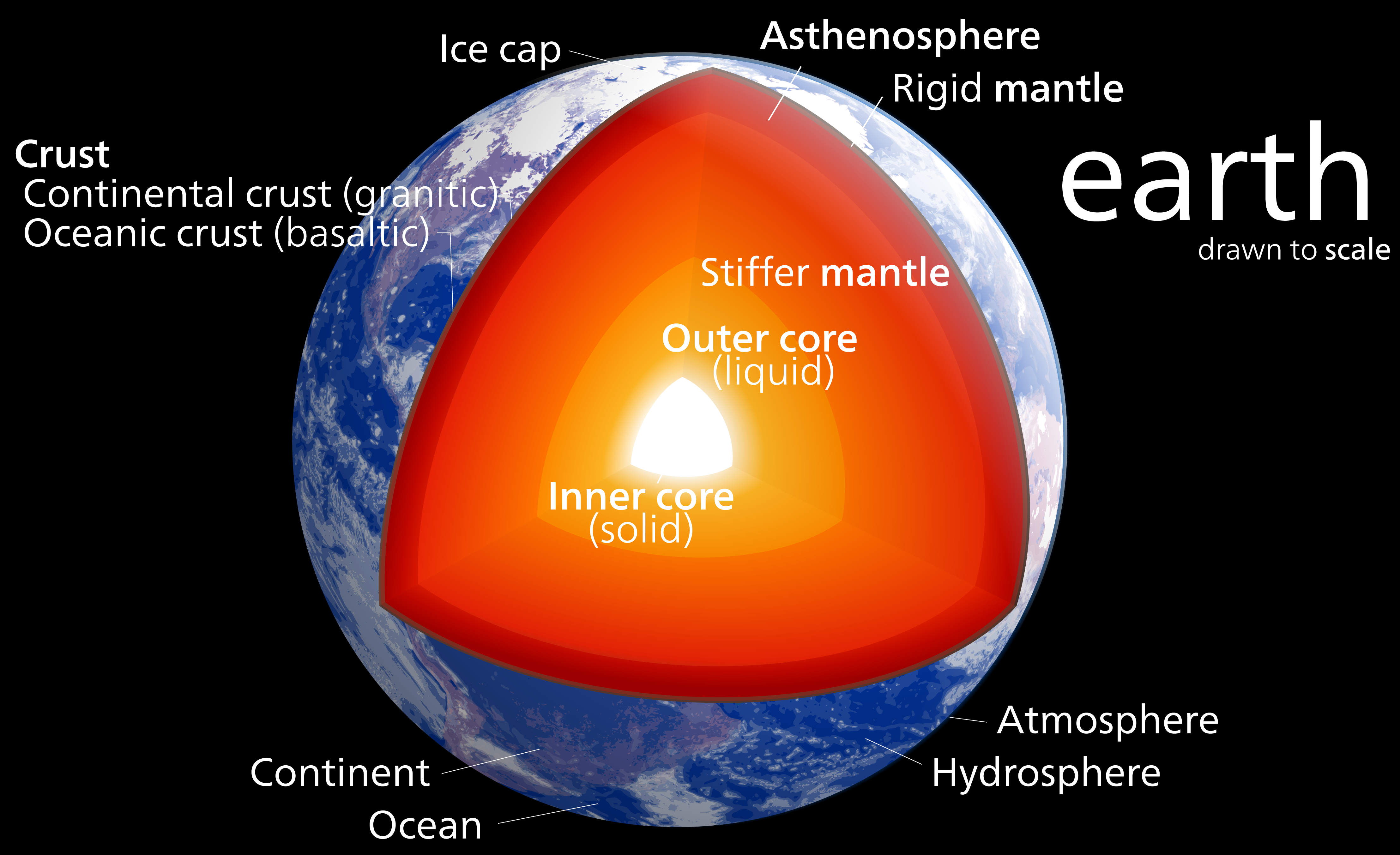
The crust in an interesting thing - it's what we live on top of and there are lots of interesting places where it's different due to geologic processes that concentrate certain types of materials. The crust is broken up into around a dozen major tectonic plates that move at about 4-6"/year. These plates are either oceanic or continental crust. Oceanic crust is generally relatively thin ~6 km (4 miles) and oceanic crust is much thicker at ~35 km (22 miles). The thin oceanic crust is also more mafic and dense than the felsic continental crust.
These differences create complex interactions when the plates meet each other at plate boundaries. We did a whole show on plate tectonics over at the Don't Panic Geocast recently, so if you'd like to hear about the discovery and arguments over plate tectonics you should check it out.
Today, I'd like to share a tool and Dr. Charles Ammon and I have made to visualize a crust model and allow anyone to explore the crust. All you need is Google Earth! We used a model called Crust 1.0 by Laske et al. that has how thick the crust (broken up into a few divisions) is for 64,800 points on the Earth along with some other crustal properties. That's every one degree of latitude and longitude! They put a lot of work into making this model. Generally we would use a Fortran program to get values out of the model, but Dr. Ammon had an idea to visualize the data in a more intuitive way with Google Earth. Over the Thanksgiving holiday I wrote a Python utility to access the model values and then we wrote a simple script that generates a Google Earth KML file based on the model.
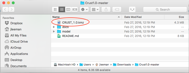
All you have to do is head over to the project's GitHub page and click the "Download ZIP" button. While you're waiting on the download you can scroll down and read all about the development, the model, and find activities to try. Next, open folder you downloaded (most operating systems will automatically unzip it for you now) there will be several files, but the only one you need is the CRUST_1.0.kmz file.
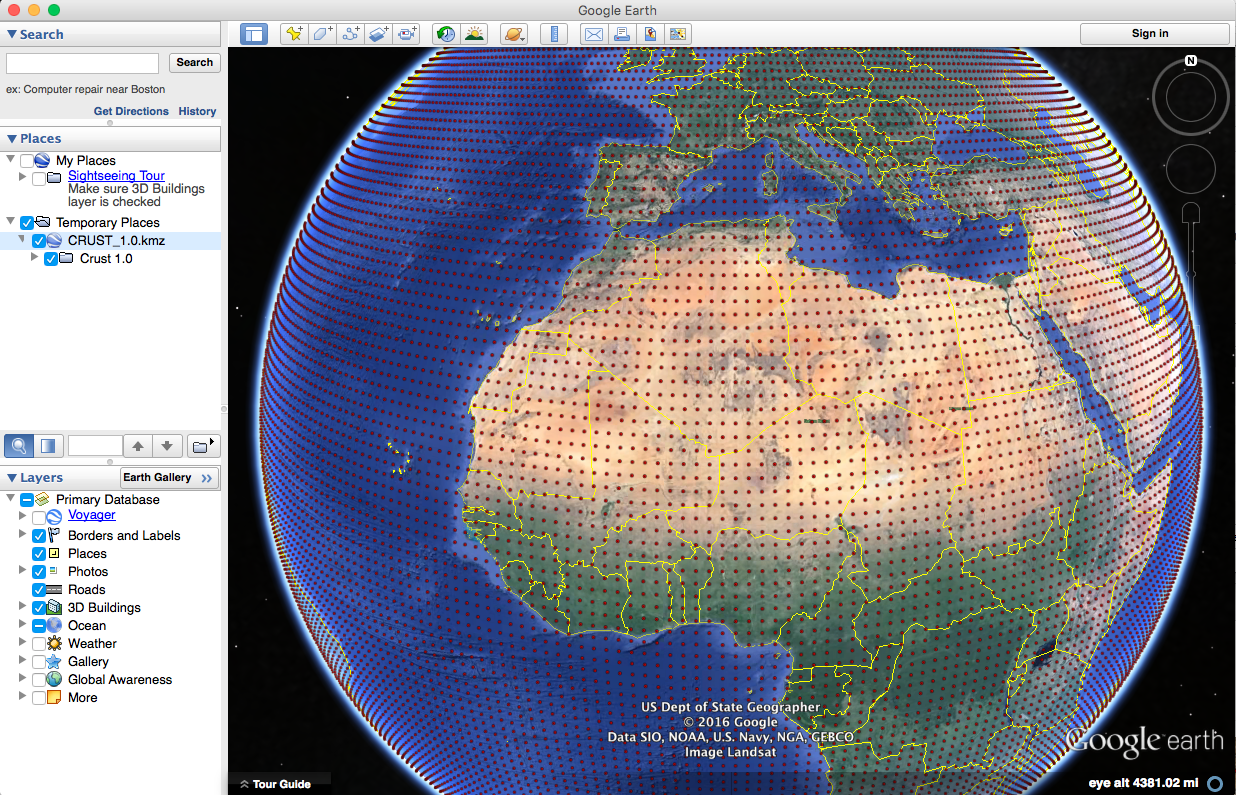
As long as you have Google Earth installed, double click that file and you'll see the Earth appear covered in red dots. If you zoom out too far, they will disappear though!
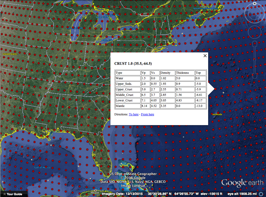
Each red dot is a location where the model has the average crustal properties like how fast P and S seismic waves can travel and the density. All of these are explained in more detail on the project webpage. You should also try some of the projects we have listed there! As a starter, let's look at oceanic and continental crust and verify my assertion about their 3x thickness difference.
Clicking out in the Atlantic Ocean (make sure you are not on the continental shelf) we see about 13 km thick crust (the top of the mantle number). The water depth is also handy to have on-hand sometimes.
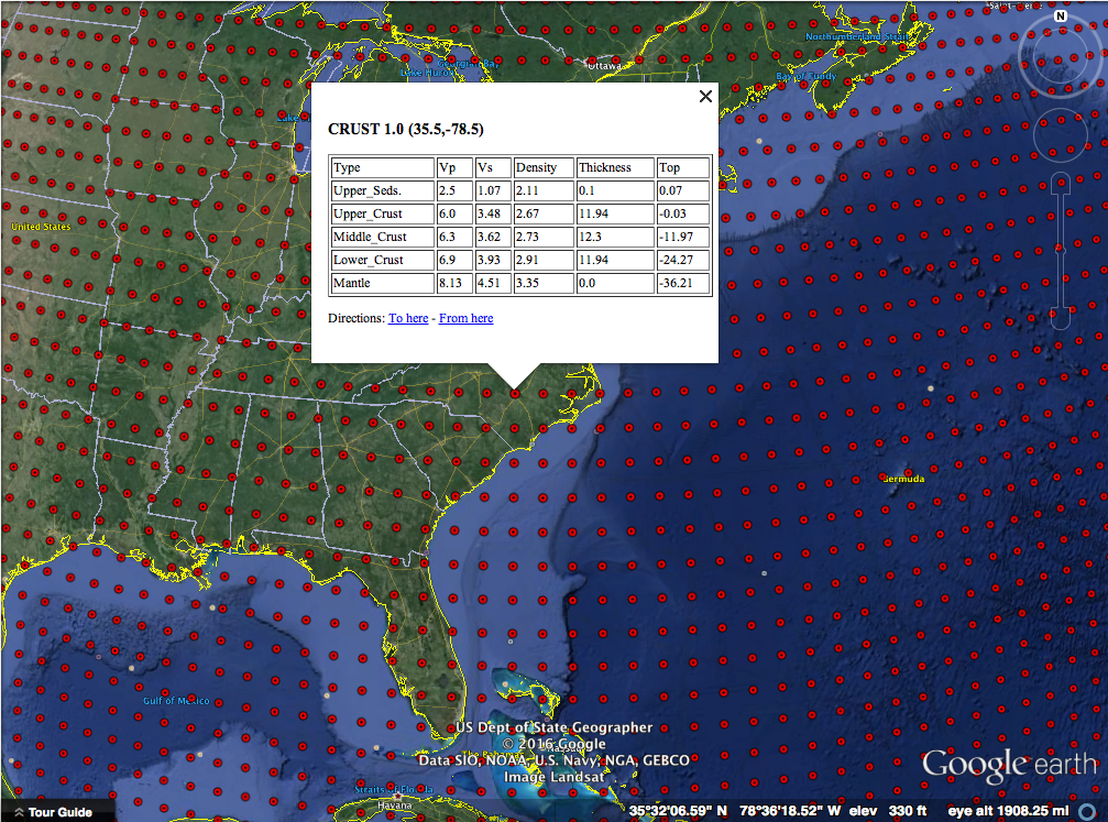
Clicking well onto the North American plate we see about 36 km thick crust. Next you should head over to mountainous regions and basins and see how the structure of the crust is different - why is that? Sorry, no homework answers here!
This is a really fun way to learn about the crust and a good reference tool as well! There are flyers in the docs folder that you can print to use as teaching aids or handout to students! We had a lot of fun making this 1-day project and hope that you'll explore it and let us know what you think! A big thanks to the folks that did the massive amount of work making the model - we just made it visible in Google Earth! Everything is open-source as always.
As frequent readers of the blog or listeners of the podcast will know, I really like doing outreach activities. It's one thing to do meaningful science, but another entirely to be able to share that science with the people that paid for it (taxpayers generally) and show them why what we do matters. Outreach is also a great way to get young people interested in STEAM (Science, Technology, Engineering, Art, Math). When anyone you are talking to, adult or child, gets a concept that they never understood before, the lightbulb going on is obvious and very rewarding.
Our lab group recently participated in two outreach events. I've shared about the demonstrations we commonly use before when talking about a local science fair. There are a few that probably deserve their own videos or posts, but I wanted to share one in particular that I improved upon greatly this year: Squeezing Rocks.
Awhile back I shared a video that explained how rocks are like springs. The normal demonstration we used was a granite block with strain gauges on it and a strip chart recorder... yes... with paper and pen. I thought showing lab visitors such an old piece of technology was a bit ironic after they had just heard about our lab being one of the most advanced in the world. Indeed when I started the paper feed, a few parents would chuckle at recognizing the equipment from decades ago. For the video I made an on-screen chart recorder with an Arduino. That was better, but I felt there had to be a better way yet. Young children didn't really understand graphs or time series yet. Other than making the line wiggle, they didn't really get the idea that it represented the rock deforming as they stepped on it or squeezed it.
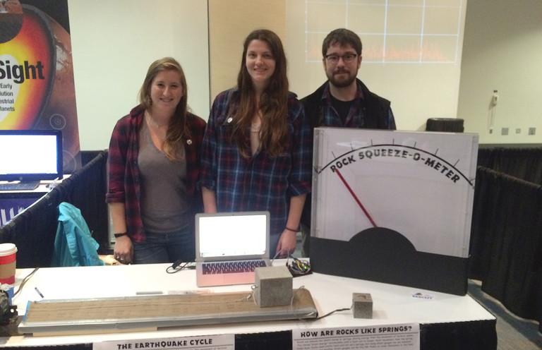
I decided to go semi old-school with a giant analog meter to show how much the rock was deformed. I wanted to avoid a lot of analog electronics as they always get finicky to setup, so I elected to go with the solution on a chip route with a micro-controller and the HX711 load cell amplifier/digitizer. For the giant meter, I didn't think building an actual meter movement was very practical, but a servo and plexiglass setup should work.
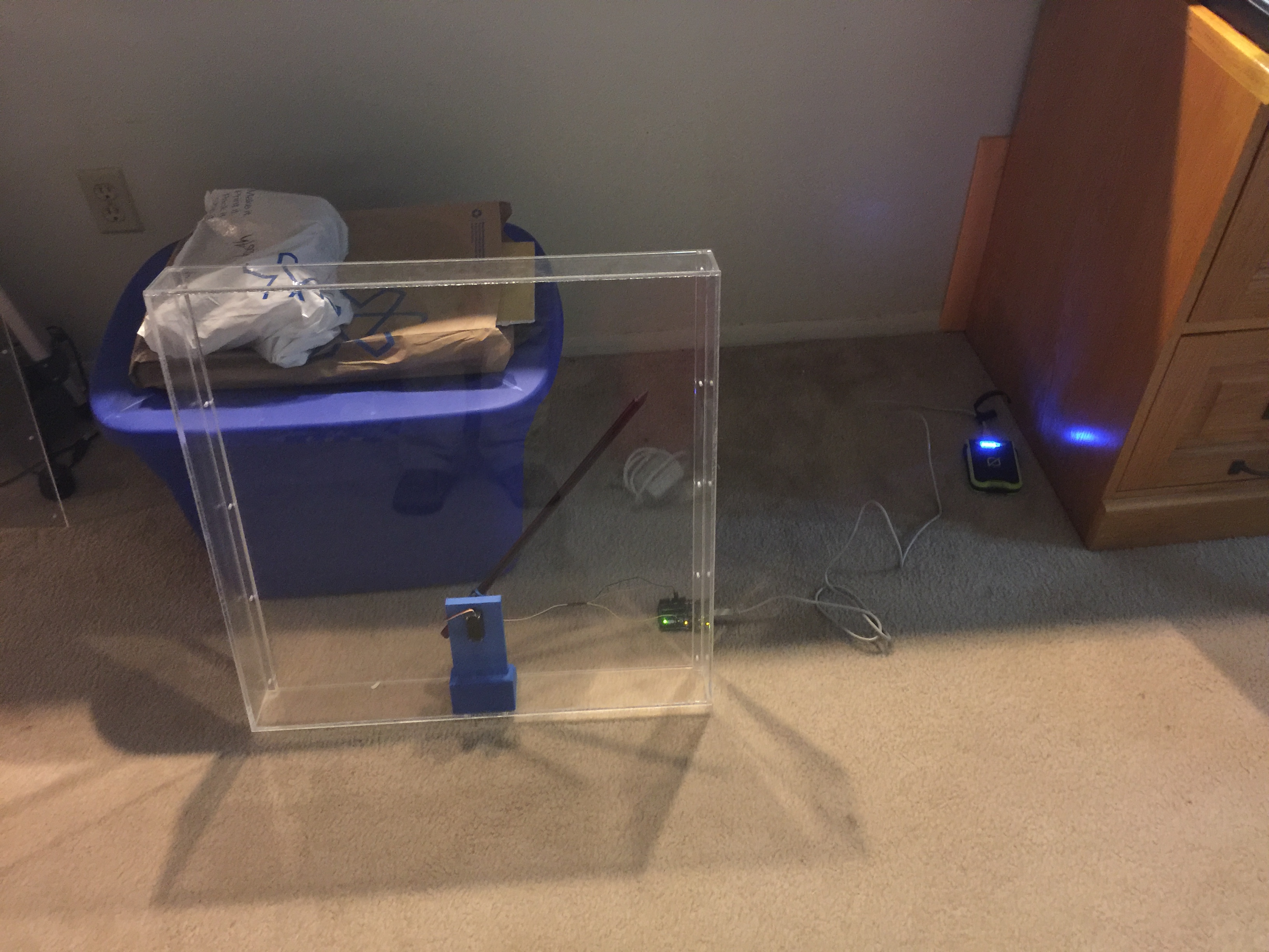
A very early test of the meters shows it's 3D printed servo holder inside and the electronics trailing behind.
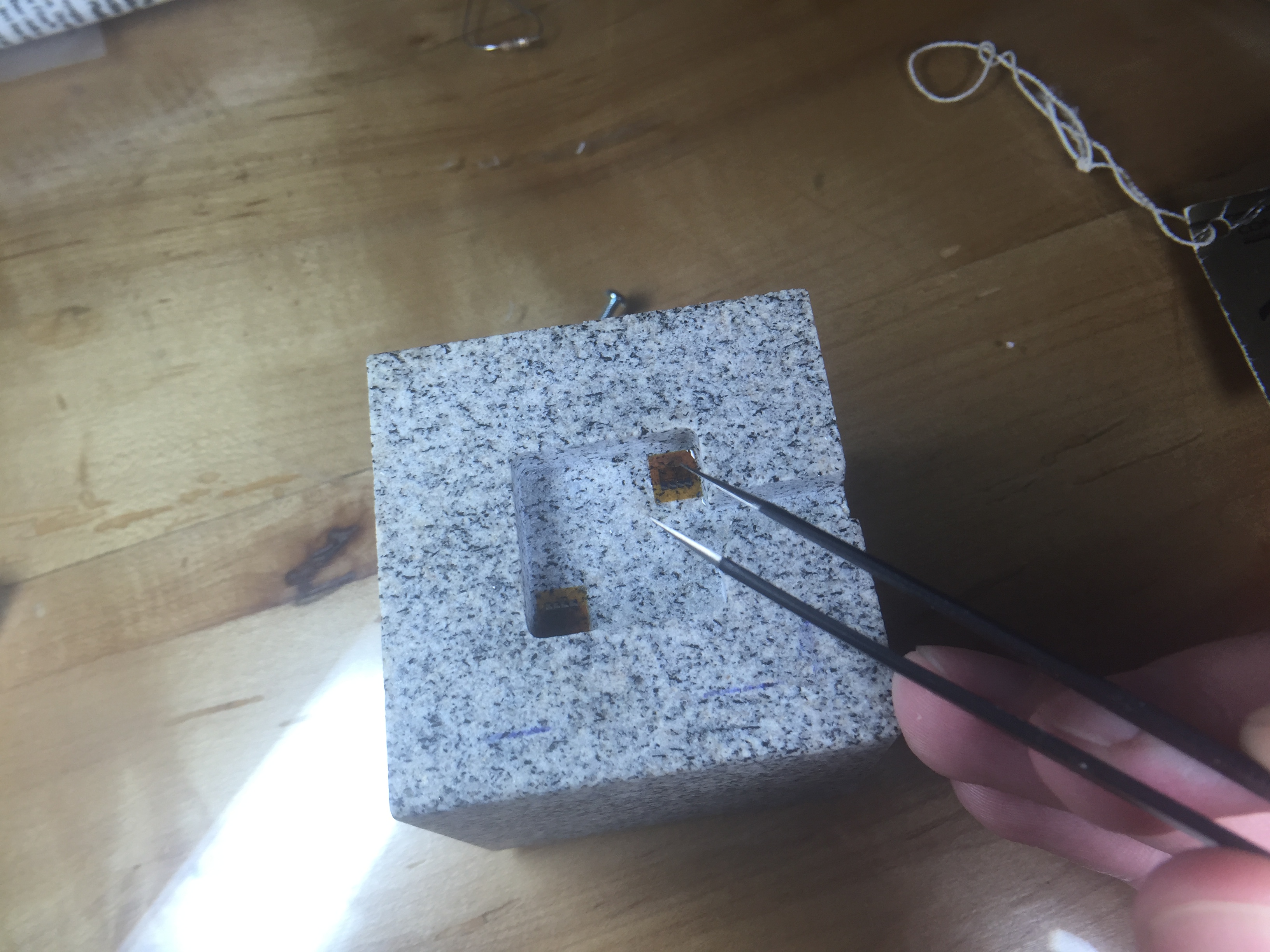
Another thing I wanted to change was the rock we use for the demo. The large granite bar you stepped on was bulky and hard to transport. I also though squeezing with your hands would add to the effect. We had a small cube of granite about 2" on a side cut with a water jet, then ground smooth. The machine shop milled out a 1/4" deep recess where I could epoxy the strain gauges.
Placing strain gauges under a magnifier with tweezers and epoxy.
Going into step-by-step build instructions is something I'm working on over at the project's Hack-a-Day page. I'm also getting the code and drawings together in a GitHub repository (slowly since it is job application time). Currently the instructions are lacking somewhat, but stay tuned. Checkout the video of the final product working below:
The demo was a great success. We debuted it at the AGU Exploration Station event. Penn State even wrote up a nice little article about our group. Parents and kids were amazed that they could deform the rock, and even more amazed when I told them that full scale on the meter was about 0.5µm of deformation. In other words they had compressed the rock about 1/40 the width of a single human hair.
A few lessons came out of this. Shipping an acrylic box is a bad idea. The meter was cracked on the side in return shipping. The damage is reparable, but I'm going to build a smaller (~12-18") unit with a wood frame and back and acrylic for the front panel. I also had a problem with parts breaking off the PCB in shipment. I wanted the electronics exposed for people to see, but maybe a clear case is best instead of open. I may try open one more time with a better case on it for transport. The final lesson was just how hard on equipment young kids can be. We had some enthusiastic rock squeezers, and by the end of the day the insulation on the wires to the rock was starting to crack. I'm still not sure what the best way to deal with this is, but I'm going to try a jacketed cable for starters.
Keep an eye on the project page for updates and if any big changes are made, you'll see them here on the blog as well. I'm still thinking of ways to improve this demo and a few others, but this was a giant step forward. Kids seeing a big "Rock Squeeze O Meter" was a real attention getter.
Hmm... As I'm writing this I'm thinking about a giant LED bar graph. It's easy to transport and kind of like those test your strength games at the fair... I think I better go parts shopping.
I end up doing a lot of debugging, in fact every single day I'm debugging something. Some days it is software and scripts that I'm using for my PhD research, some days it is failed laboratory equipment, and some days it's working the problems out of a new instrument design. Growing up working on mechanical things really helped me develop a knack for isolating problems, but this is not knowledge that everyone has the occasion to develop. I'm always looking for ways to help people learn good debugging techniques. There's nothing like discovering, tracking down, and fixing a bug in something. Also, the more good debuggers there are in the world, the fewer hours are waisted fruitlessly guessing at problems.
I'd heard about a debugging book that was supposed to be good for any level of debugger, from engineer to manager to homeowner. I was a little suspicious since the is such a wide audience, but I found that my library had the book and checked it out; it is "Debugging: The 9 Indispensable Rules for Finding Even the Most Elusive Software and Hardware Problems" by David Agans. The book sat on my shelf for a few months while I was "too busy" to read it. Finally, I decided to tackle a chapter a day. The chapters are short and I can handle two weeks of following the book. Each morning when I got to work, I read the chapter for that day. One weekend I read an extra chapter or two because they were enjoyable.
I'm not going to ruin the book, but I am going to tell you the 9 rules (it's okay, they are also available in poster form on the book website).
Understand the System
Make It Fail
Quit Thinking and Look
Divide and Conquer
Change One Thing at a Time
Keep an Audit Trail
Check the Plug
Get a Fresh View
If You Didn't Fix It, It Ain't Fixed
They seem simple, but think of the times you've tried to fix something and skipped around because you thought you knew better to have it come back to sting you. If you've done a lot of debugging, you can already see the value of this book.
The book contains a lot of "war stories" that tell tales of when a rule or several rules were the key in a debugging problem. My personal favorite was the story about a video conferencing system that seemed to randomly crash. Turns out the compression of the video had problems with certain patterns and when the author wore a plaid shirt to work and would test the system, it failed. He ended up sending photocopies of his shirt to the manufacturer of the chip. Fun stories like that made the book fun to read and show how you have to pay attention to everything when debugging.
The book has a slight hardware leaning, but has examples of software, hardware, and home appliances. I think that all experimentalists or engineers should read this early on in their education. It'll save hours of time and make you seem like a bug whisperer. Managers can learn from this too and see the need to provide proper time, tools, and support to engineering.
If you like the blog, you'll probably like this book or know someone that needs it for Christmas. I am not being paid to write this, I don't know the author or publisher, but wanted to share this find with the blog audience. Enjoy and leave any comments about resources or your own debugging issues!
Today I wanted to share some thoughts on some great new technology that is being actively developed and uses cameras to extract sound and physical property information from everyday objects. I had heard of the visual microphone work that Abe Davis and his cohorts at MIT were working with, but they've gone a step further recently. Before we jump in, I wanted to thank Evan Bianco of Agile Geoscience for pointing me in this direction and asking about what implications this could have for rock mechanics. If you like the things I post, be sure to checkout Agile's blog!
Abe's initial work on the "visual microphone" consisted of using high speed cameras and trying to recover sound in a room by videoing an object like a plant or bag of chips and analyzing the tiny movements of the object. Remember sound is a propagating pressure wave and makes things vibrate, just not necessarily that much. I remember thinking "wow, that's really neat, but I don't have a high speed camera and can't afford one". Then Abe figured out a way to do this with normal cameras by utilizing the fact that most digital cameras have a rolling shutter.
Most video cameras around shoot video at 24 or 32 frames (still photos) each second (frames per second or fps). Modern motion pictures are produced at 24 fps. If we change the photos very slowly and we just see flashing pictures, but around the 16 fps mark our mind begins to merge the images into a movie. This is an effect of persistence of vision and it's a fascinating rabbit hole to crawl down. (For example, did you know that old time film projectors flashed the same frame more than once? The rapid flashing helped us not see flickers, but still let the film run at a slower speed. Checkout the engineer guy's video about this.) In the old days of film, the images were exposed all at once. Every point of light in the scene simultaneously flooded through the camera and exposed the film. That's not how digital cameras work at all. Most digital cameras use a rolling shutter. This means the image acquisition system scans across the CCD sensor row by row (much like your TV scans to show an image, called raster scanning) and records the light hitting that sensor. This means for things moving really fast, we get some strange recordings! The camera isn't designed to capture things that move significantly in a single frame. This is a type of non-traditional signal aliasing. Regular aliasing is why wagon wheels in westerns sometimes look like they are spinning backwards. Have a look at the short clip below that shows an aircraft propeller spinning. If that's real I want off the plane!
But how does a rolling shutter help here? Well 24 fps just isn't fast enough to recover audio. A lot of audio recordings sample the air pressure at the microphone about 44,200 times per second. Abe uses the fact that the scanning of the sensor gives him more temporal resolution than that rate at which entire frames are being captured. The details of the algorithm can get complex, but the idea is to watch an object vibrate and by measuring the vibration estimate the sound pressure and back-out the sound.
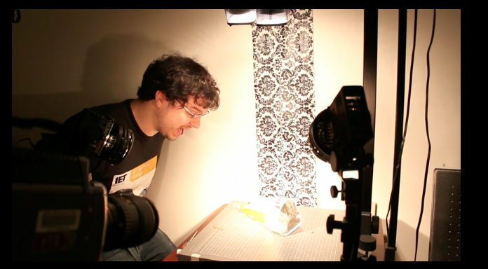
Sure we've all seen spies reflect a laser off glass in a building to listen to conversations in the room, but this is using objects in the room and simple video! Early days of the technology required ideal lighting and loud sounds. Here's Abe screaming the words to "Mary had a little lamb" at a bag of potato chips for a test.... not exactly the world of James Bond.
As the team improved the algorithm, they filmed the bag in a natural setting through a glass pane and recovered music. Finally they were able to recover music from a pair of earbuds laying on a table. The audio quality isn't perfect, but good enough that Shazam recognized the song!
The tricks that the group has been up to lately though are what is the most fascinating. By videoing objects that are being minority perturbed by external forces, they are able to model the object's physical properties and predict its behavior. Be sure to watch the TED talk below to see it in action. If you're short on time skip into about the 12 minute mark, but really just watch it all.
By extracting the modulus/stiffness of objects and how they respond to forces, the models they create are pretty lifelike simulations of what would happen if you exerted a force on the real thing. The movements don't have to be big. Just tapping the table with a wire figure on it or videoing trees in a gentle breeze is all it needs. This technology could let us create stunning effects in movies and maybe even be implemented in the lab.
I've got some ideas on some low hanging fruit that could be tried and some more advanced ideas as well. I'm going to talk about that next time (sorry Evan)! I want to make sure we all have time to watch the TED video and that I can expand my list a little more. I'm thinking along the lines of laboratory sensing technology and civil engineering modeling on the cheap... What ideas do you have? Expect another post in the very near future!
It is finally summer and I see lots of people playing all sorts of outdoor sports. While I have never been a big sports player, it is fun to watch. There are a lot of physics involved in most sports, so maybe that is a line of posts worth investigating. I do have a post series on open source science planned that will last most of the summer, but maybe we can keep sports in mind next year?
This post is a resurrection of a post I started a couple of years ago and never got around to finishing. In an effort to tie up loose ends, here we go! How does a frisbee fly? I wondered this when we discovered that my fiancée can throw a frisbee upside down sometimes with results that flew surprisingly far. To understand what is happening we need to look at the fundamental physics of frisbee flight, make some measurements, then try to draw some conclusions. Turns out there is a lot of research on the aerodynamics of flying discs, so I'll hit the important points and leave links to let you dig down the wiki-hole with me if you wish. To start out, check out a copy of "Spinning Flight" by Ralph Lorenz at your library.
The physics of frisbee flight
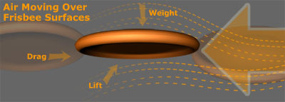
While in flight, our frisbee will experience several forces governing its movement including gravity, lift, drag, and a torque from its angular momentum. We will quickly look at each of these, but we are not going to fully model the system (though it could be fun!)
Forces on a frisbee. (Image: illumin.usc.edu)
First off, Gravity is the most obvious and intuitive of these forces. Everything is pulled towards the earth's center of mass by gravity at about 9.81m/s/s. If we just place the frisbee on the table, it will experience a force resulting from the acceleration of gravity. If we drop it, it will be accelerated downward. The velocity of falling objects has been fully investigated and we won't go into that too deeply. For now, simply assume that we could calculate the velocity of a dropped object or calculate the acceleration of an object if we know its fall rate.
Lift is what may be the most important force in this study. Believe it or not, a frisbee experiences lift following the same principles as a traditional wing or rotor blade. As the frisbee cuts through the air, some of the oncoming air goes over the frisbee, some goes under. The air streams have to meet up in the lee of the frisbee and since we cannot create or destroy air, we must have continuity and conservation. The air on top has to move faster for this to hold, it has longer to travel after all, and the air below can move more slowly. Thanks to Bernoulli's principle, we know that air moving faster will have a decreased pressure. This isn't anything new; in fact, Daniel Bernoulli published this idea in 1738! With fast air on top of the frisbee and slower air below, there is high pressure below and low pressure above the disk. From a difference in pressure we get the force of lift (more generally called a pressure gradient force).
Lift force from a pressure differential. (Image web.wellington.org)
Drag is the reason that our frisbee does not fly off into the distance. Drag is the force that slows the frisbee down as it pushes through the dense atmosphere. We could try to measure the drag through our later analysis, but that itself it a very deep task that we could spend a lot of time on.
Finally, comes the torque from the angular momentum of our frisbee. Have you tried to throw a frisbee without spinning it? In theory it would fly right? It's just a circular wing after all. Well, that turns out to be a pretty unstable way to fly your disc. Generally it will turn up, stall, and then fall like a rock. Why? Thanks to some spatial change in the lift force, the front of the disc will be lifted with slightly more force than the back, causing the disc to torque over to the back. In fact, I'll save you the trouble, you can watch my feeble attempts below. We could try to outfit our frisbee with control surfaces to help it maintain the proper angle of attack, but that is heavy, complicated, and would mean dead batteries would plague playing kids and dogs. Surely there is a more simple way?
Of course! Let's spin the frisbee when we throw it! When we throw the disc and it spins, we get gyroscopic stability and the possibility to see the cool spinning designs we print on the toy. We can determine that this torque will point vertically through the top of the frisbee. If you remember the right hand rule, you'll see that for my right-handed clockwise throw, the torque vector will point towards the ground. For the south-paws out there, your torque vector will point towards the sky. The important thing is that it will try to counteract the tendency of the lift moment to make the frisbee backflip. Granted, it will not win forever. Eventually the flight will become unstable, but we can maintain steady flight for several seconds. Depending on the force balance, we'll also expect to see the frisbee's vertical axis precess around true "up".
Taking measurements
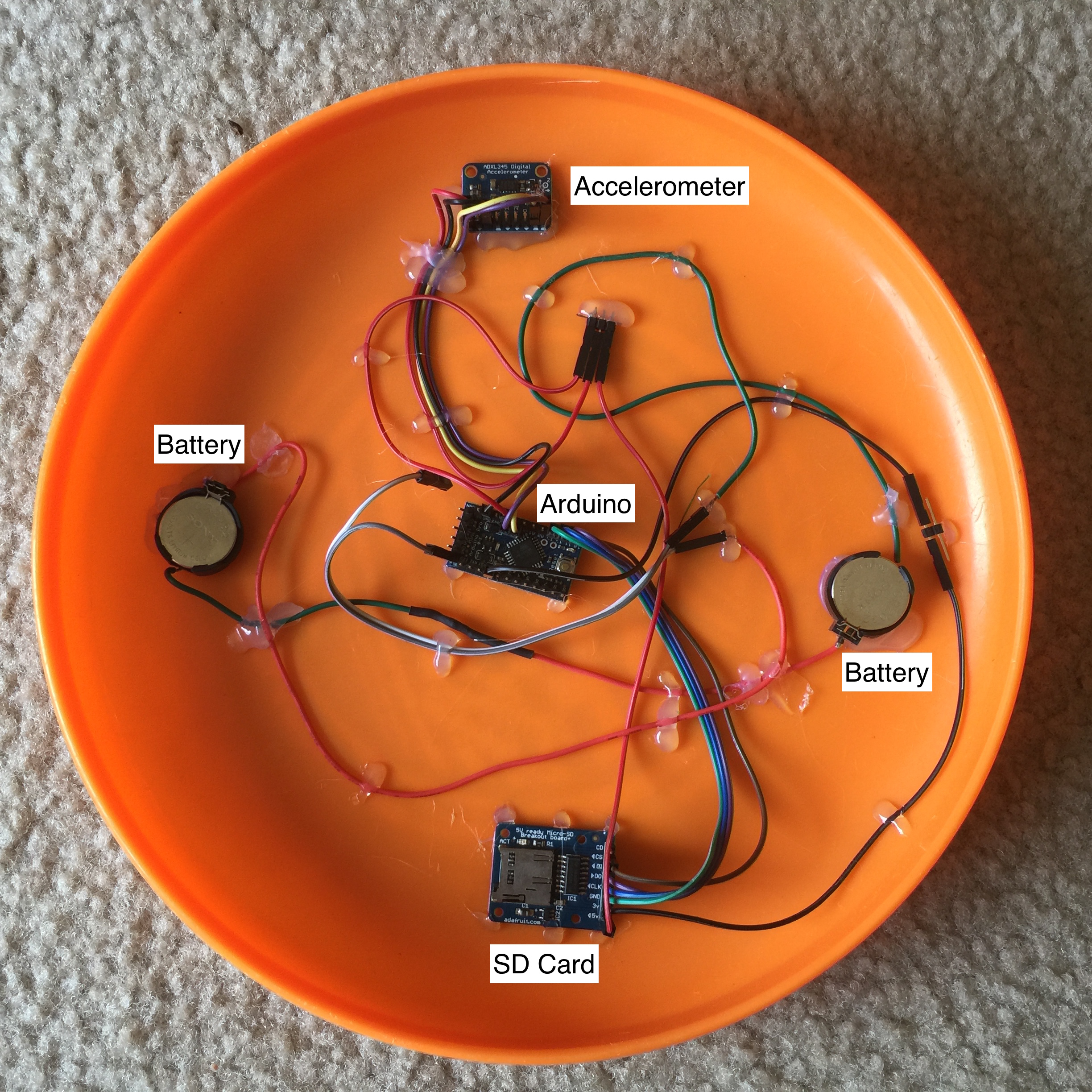
To take some measurements of frisbee flight, I created an instrumented frisbee. Turns out, I'm not the first one to do this. Lorenz made an instrumented frisbee in the early 2000's and then improved it by adding a plethorera of sensors. I decided that a simple accelerometer would be enough for my investigation. While adding angle sensors and such would be interesting, let's keep it simple for a first pass. Maybe adding a 9 degree of freedom inertial measurement unit would be fun, but that's an idea for another time. Actually, the gyroscope data from that would be incredibly useful.
I used an Arduino Pro Mini for my micro controller, an accelerometer, and SD card logger for the sensor and logging system. I ended up just trying to read the sensor in single shot mode as fast as possible. This gave a data rate of around 180-200 Hz with time-stamps in microseconds on each packet. Sure, we could make this part a little more slick, but again, the KISS principle rules for these first hacks at a problem . Power comes from a pair of CR2032 coin cell batteries. All of this was hot glued down and hopefully made as aerodynamic as possible without coweling the whole assembly. Should we wish to improve this, I would directly solder the wires to the boards instead of using header connectors and cover everything in kapton tape.
If you are interested in trying this yourself, the Arduino sketch is at the bottom of this post.
To approximate the speed of the frisbee I will have some video of the flights that we can look at to get some rough numbers to work with. These were just filmed with a DSLR camera, so this is something you can try at home! The newer iPhones are actually even faster than this camera, but I didn't have a tripod mount handy for my 6+ when I filmed this.
Data analysis
First, let's look at the film of a flight to figure out how fast the frisbee throw is on average. We could look at how long the flight was and how far is was and get an average velocity with v=d/t. That's great, but we can do one better! Through the magic of image tracking, we can get the position of the frisbee in each frame of the video and calculate the velocity profile during the flight. While probably not totally necessary, why not?
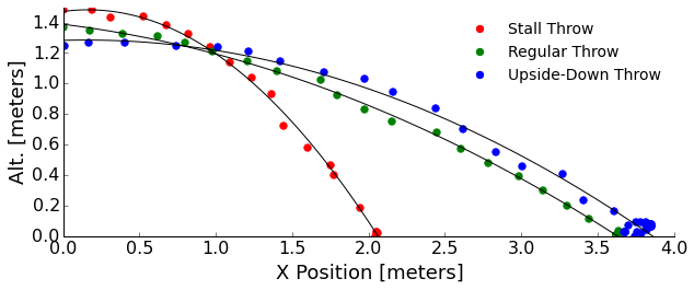
I'll use the Tracker video analysis software for this. We read in the video, setup some coordinate systems, markers, etc, and let it churn. If the frisbee veers in the third dimension (into or out of the screen) we won't get that information because we are just tracking its center in a 2D picture. Hence, I'll try to keep the throws gentle! We'll look at the stall, upside-down, and normal throws:
To keep this short, I'll tell you that the forward speed of these throws looks to top out at about 5 m/s. Again, we could go down the hole of getting drag from the slight deceleration in forward speed with time, but it really doesn't slow us much... the ground beats drag to stopping our frisbee.
We can see that the stall throw drops very quickly without really flying. In fact, it mostly is flipping end-over-end. The regular and upside-down throws look like they have a similar flight profile from the video. This means I must have not been as consistent as I had hoped with my throwing strength. We know that without the lift component that the upside-down throw should follow a more parabolic path than the regular throw. Also, my regular throw was pretty weak to keep the frisbee in the frame and minimally veering, so it didn't have enough lift to show us long periods of stable flight.
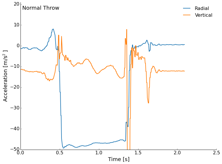
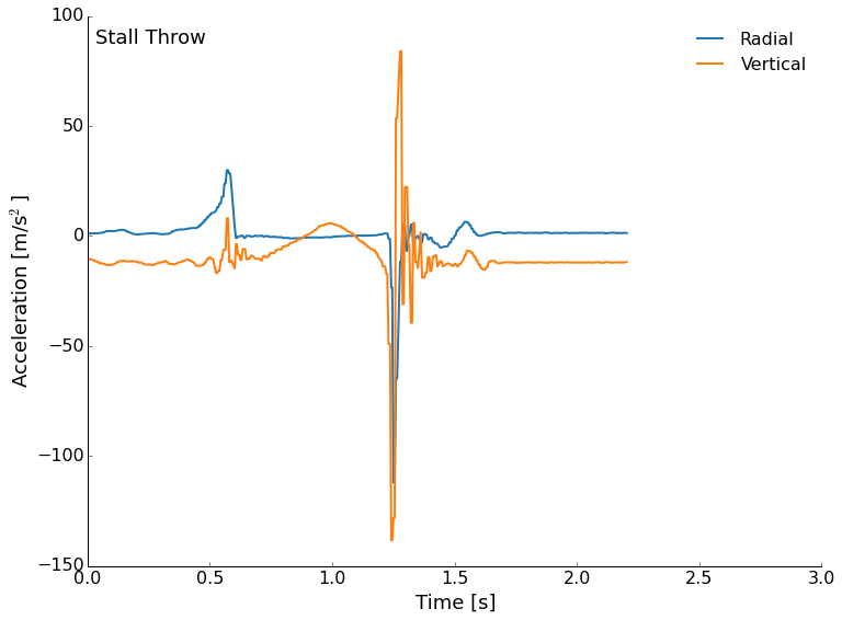
Next, let's look at the accelerometer data. The data is stored in a text file with the millisecond time stamp, and then each of the three axes acceleration measurements. I've plotted the radial (outward from the center) and vertical accelerations. Since the accelerometer was mounted near the rim of the frisbee, we will see relatively large signals from the wobble in flight.
We'll start with the normal throw this time. The accelerometer is roughly calibrated at the factory, but don't worry about the absolute values too much here. We see me pull back to throw as a upturn in the radial, then a large negative (outward) acceleration from the spinning of the disc during flight. Roughly a couple of g's here. The vertical is interesting through. We see the roughly -10m/s/s from the Earth's gravity as a prepare to throw and after the landing, but during flight we see a near zero vertical acceleration that trends downward. What is it? Lift! This is the flight of the frisbee that is gradually reduced as drag slows us and the angle of attack becomes non-ideal. We are expecting that we don't totally counteract gravity because flight is not sustained and our frisbee does not go on forever. This was a pretty gentle and short flight, but followed our expectations in terms of the forces at work. We can even see some precession in the vertical in the neighborhood of about 4 times/second.
Next, we'll look at the stall throw. This isn't spinning so we don't expect to see a lot of radial acceleration once the throw leaves our hands, but we do expect to see some lift for a short period of time, then a stall and fall. That is what we get, too! The spike in the blue curve at 0.5 seconds is my push to accelerate the frisbee, then there are few other radial accelerations recorded (except the impact). There should be some small accelerations from the flip of the disc, but they are tiny here. The vertical trend up and down just before 1 second is the frisbee flipping over once. The only real lift is just a tiny fraction of a second before the front is lifted up. After that, we are really just in free-fall.
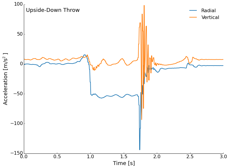
Finally, the elusive upside-down throw. The frisbee starts out upside-down, so the acceleration of gravity now shows as positive (look after the landing for example). We still see radial acceleration from the spinning and we also see a reduction in the vertical acceleration. This can't be lift, but is probably some axis mis-alignment on the sensor. We still see precession as the torque tries to keep the disc horizontal.
What did we learn?
We learned about all of the forces at play in the flight of a frisbee, lift, drag, etc. We measured some flight paths and acceleration profiles. These were not quite as clear cut as I had hoped though. We still saw that flying right side up works pretty well, but upside down "flight" is basically spin-stabilized falling with a lot of forward momentum. Throwing with no spin quickly results in a pitch-up and stall.
We'll see what happens with this. If people are interested we could think about adding an IMU to the setup with better positioning and balance. We could also just put a light on a frisbee and track it with a time-lapse photo. This turned out to be a fascinating look at flight, acceleration measurement, and video tracking! If you are wondering about numerical modeling, there is a really nice report from MIT that develops a good model.
#include <SPI.h>
#include <SD.h>
#include <Wire.h>
#include <Adafruit_Sensor.h>
#include <Adafruit_ADXL345_U.h>

/* Assign a unique ID to this sensor at the same time */
Adafruit_ADXL345_Unified accel = Adafruit_ADXL345_Unified(12345);

const int chipSelect = 4;

File dataFile;

void displaySensorDetails(void)
{
sensor_t sensor;
accel.getSensor(&sensor);
Serial.println("------------------------------------");
Serial.print ("Sensor: "); Serial.println(sensor.name);
Serial.print ("Driver Ver: "); Serial.println(sensor.version);
Serial.print ("Unique ID: "); Serial.println(sensor.sensor_id);
Serial.print ("Max Value: "); Serial.print(sensor.max_value); Serial.println(" m/s^2");
Serial.print ("Min Value: "); Serial.print(sensor.min_value); Serial.println(" m/s^2");
Serial.print ("Resolution: "); Serial.print(sensor.resolution); Serial.println(" m/s^2");
Serial.println("------------------------------------");
Serial.println("");
delay(500);
}

void displayDataRate(void)
{
Serial.print ("Data Rate: ");

switch(accel.getDataRate())
{
case ADXL345_DATARATE_3200_HZ:
Serial.print ("3200 ");
break;
case ADXL345_DATARATE_1600_HZ:
Serial.print ("1600 ");
break;
case ADXL345_DATARATE_800_HZ:
Serial.print ("800 ");
break;
case ADXL345_DATARATE_400_HZ:
Serial.print ("400 ");
break;
case ADXL345_DATARATE_200_HZ:
Serial.print ("200 ");
break;
case ADXL345_DATARATE_100_HZ:
Serial.print ("100 ");
break;
case ADXL345_DATARATE_50_HZ:
Serial.print ("50 ");
break;
case ADXL345_DATARATE_25_HZ:
Serial.print ("25 ");
break;
case ADXL345_DATARATE_12_5_HZ:
Serial.print ("12.5 ");
break;
case ADXL345_DATARATE_6_25HZ:
Serial.print ("6.25 ");
break;
case ADXL345_DATARATE_3_13_HZ:
Serial.print ("3.13 ");
break;
case ADXL345_DATARATE_1_56_HZ:
Serial.print ("1.56 ");
break;
case ADXL345_DATARATE_0_78_HZ:
Serial.print ("0.78 ");
break;
case ADXL345_DATARATE_0_39_HZ:
Serial.print ("0.39 ");
break;
case ADXL345_DATARATE_0_20_HZ:
Serial.print ("0.20 ");
break;
case ADXL345_DATARATE_0_10_HZ:
Serial.print ("0.10 ");
break;
default:
Serial.print ("???? ");
break;
}
Serial.println(" Hz");
}

void setup(void)
{
Serial.begin(9600);
Serial.println("Accelerometer Test"); Serial.println("");

/* Initialise the sensor */
if(!accel.begin())
{
/* There was a problem detecting the ADXL345 ... check your connections */
Serial.println("Ooops, no ADXL345 detected ... Check your wiring!");
while(1);
}

/* Set the range to whatever is appropriate for your project */
accel.setRange(ADXL345_RANGE_16_G);
// displaySetRange(ADXL345_RANGE_8_G);
//accel.setRange(ADXL345_RANGE_4_G);
// displaySetRange(ADXL345_RANGE_2_G);

/* Display some basic information on this sensor */
displaySensorDetails();

/* Display additional settings (outside the scope of sensor_t) */
displayDataRate();
//displayRange();
Serial.println("");
Serial.print("Initializing SD card...");
// make sure that the default chip select pin is set to
// output, even if you don't use it:
pinMode(SS, OUTPUT);

// see if the card is present and can be initialized:
if (!SD.begin(chipSelect)) {
Serial.println("Card failed, or not present");
// don't do anything more:
while (1) ;
}
Serial.println("card initialized.");

char filename[15];
strcpy(filename, "ACCLOG00.TXT");
for (uint8_t i = 0; i < 100; i++) {
filename[6] = '0' + i/10;
filename[7] = '0' + i%10;
// create if does not exist, do not open existing, write, sync after write
if (! SD.exists(filename)) {
break;
}
}

dataFile = SD.open(filename, FILE_WRITE);
if( ! dataFile ) {
Serial.print("Couldnt create ");
Serial.println(filename);
while(1);
}
Serial.print("Writing to ");
Serial.println(filename);
}

void loop(void)
{
/* Get a new sensor event */
for(int i=0; i < 100; i++){
sensors_event_t event;
accel.getEvent(&event);
dataFile.print(millis());
dataFile.print(",");
//log_float(event.acceleration.x,999,8,5);
dataFile.print(event.acceleration.x,5);
dataFile.print(",");
//log_float(event.acceleration.x,999,8,5);
dataFile.print(event.acceleration.y,5);
dataFile.print(",");
//log_float(event.acceleration.x,999,8,5);
dataFile.print(event.acceleration.z,5);
dataFile.println("");
}
dataFile.flush();
}
I had been thinking about a blog post on the importance of being a mentor in an academic setting (or any other setting really). Unfortunately I lost one of my early mentors and wanted to write a short story to show the impact that being a mentor can have.
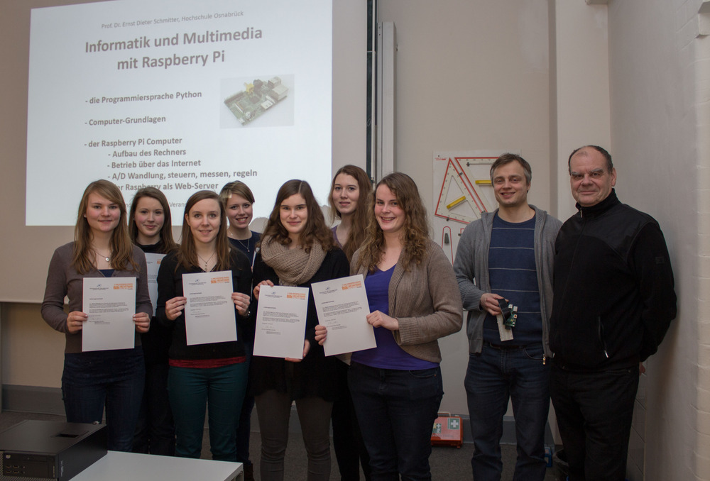
When I was in high-school I was fascinated by tornadoes and electric fields. I still am. I decided that I wanted to research the connection, so I began to read lots of literature on the subject (my first exposure to peer-reviewed papers) and looking for places I could contribute. I landed on the Yahoo Groups page of a group dedicated to ULF/VLF studies. After asking some very basic questions, I ended up chatting with Prof. Schmitter through e-mail. After weeks of communication and beginning to design an instrument, he inquired as to which institution I was at. I replied that I was a high school student, expecting to never hear back from him. The response was exactly the opposite. Ernst re-doubled his efforts to help me undertake a project.
This effort wasn't to check off a box on a funding agency outreach goal sheet, but it was a true excitement to help a student learn. I was very excited about the whole thing! We did design an instrument that I constructed at my home in Arkansas. Some friends and I took it to the field and collected data. After returning, I sent Ernst the data and he suggested we write a publication.
Having never written anything more than a detailed physics lab report before, this was an incredible learning experience. We worked the paper over a few times and had a couple of Skype calls about it. He submitted the paper, absorbing the cost of publication. That was my first scientific article.
Did I mention that he was a professor in Germany? We never met in person. I had seen his recent publications come out and kept meaning to email and update him that I had again been working in electrostatics. I didn't get it done. It had been too many years since we talked. I do have a new instrument that we designed some years ago that still needs to be built and tested, but it will surely be many times more difficult now.
What is the lesson in this other than contacting people before you can't anymore? It's is that you never know who you will inspire. Without pushes from Prof. Schmitter I probably wouldn't have finished the project and published anything. That publication helped me get a foot in the door of the research field. That's how I found out I wanted to do research as a career (thanks to several other amazing mentors). The lesson is that taking the time to talk to interested students is one way to have a lasting impact, even after your time.
I consider myself incredibly lucky to have had as many amazing mentors and teachers at every stage of my life. I'm in much deeper service debt than I can ever hope to pay off in one lifetime. I want to thank everyone reading this for encouraging me through direct contact or just by supporting this blog with your readership. This post serves to show that everyone of you make a difference in the lives of others everyday.
* I looked back through our emails had we had nearly 200 pages of email exchange before I had finished my first year of college. That's a lot of information!
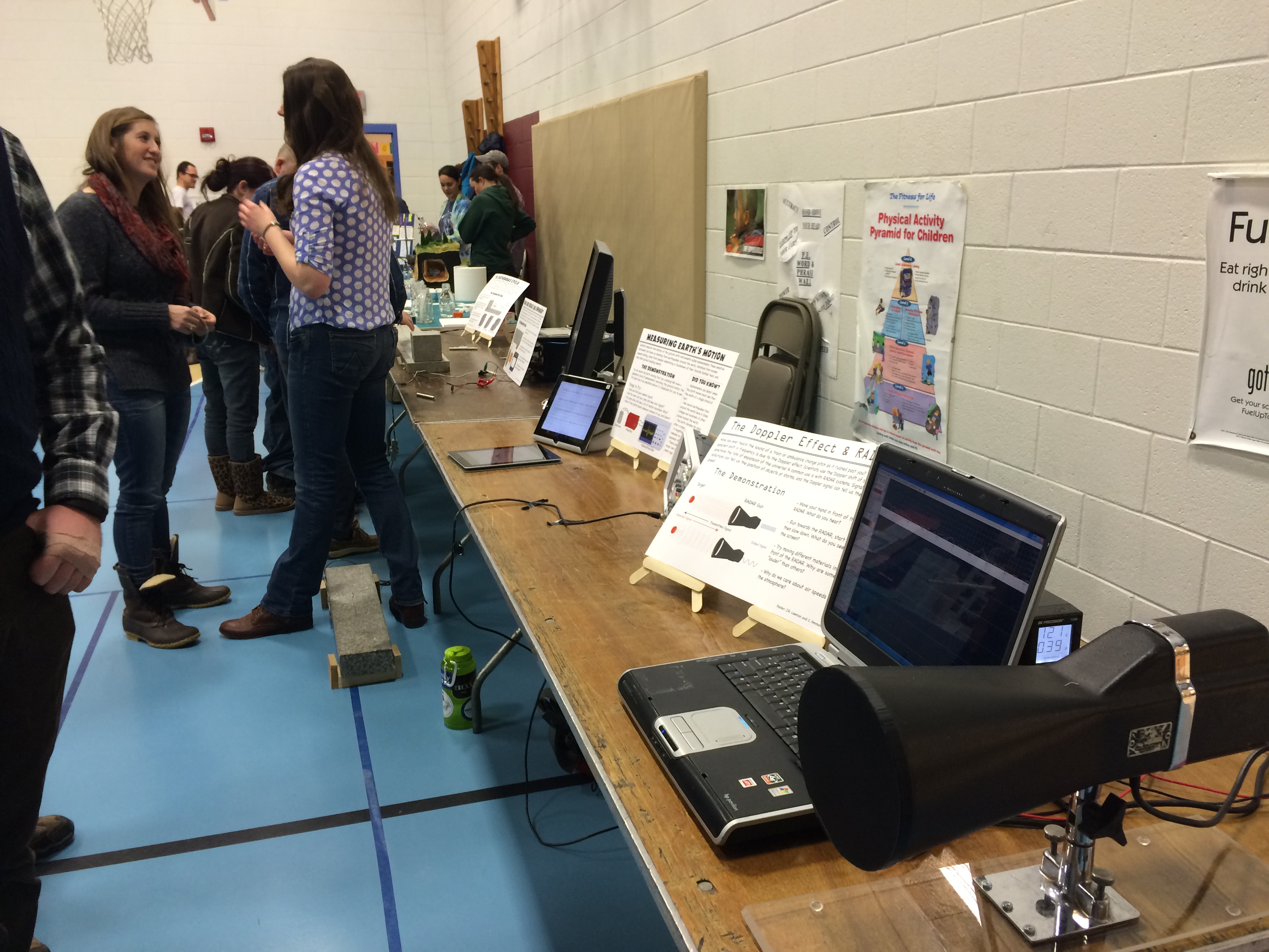
This past week I got to relive some of my favorite days of primary education: the science fair! A local elementary school was hosting their annual science fair and had asked the department to provide some demonstrations for the parents and students to see. I immediately volunteered our lab group and began to gather up the required materials. Some of the setups were made years ago by my advisor. I also developed a few and improved upon others here and there. I thought it would be fun to share the experience with you.
The line-up of demonstrations setup as the science fair was getting started.
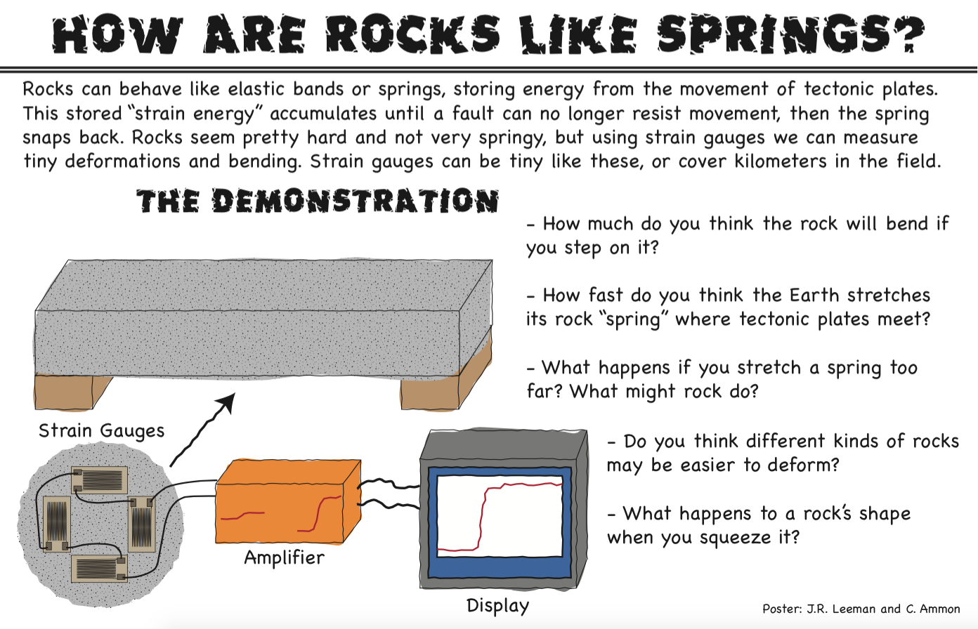
At some point, we should probably have a post or two about each of these demonstrations, but today we'll look at pictures and talk about the general feedback I received. First, off we had four demonstrations including the earthquake cycle, how rocks are like springs, seismometers, and Doppler RADAR. I made an 11x17" poster for each demo in Adobe Illustrator using a cartoon technique that one of our professors here shared with me.
Here is an example poster from one of the demonstrations.
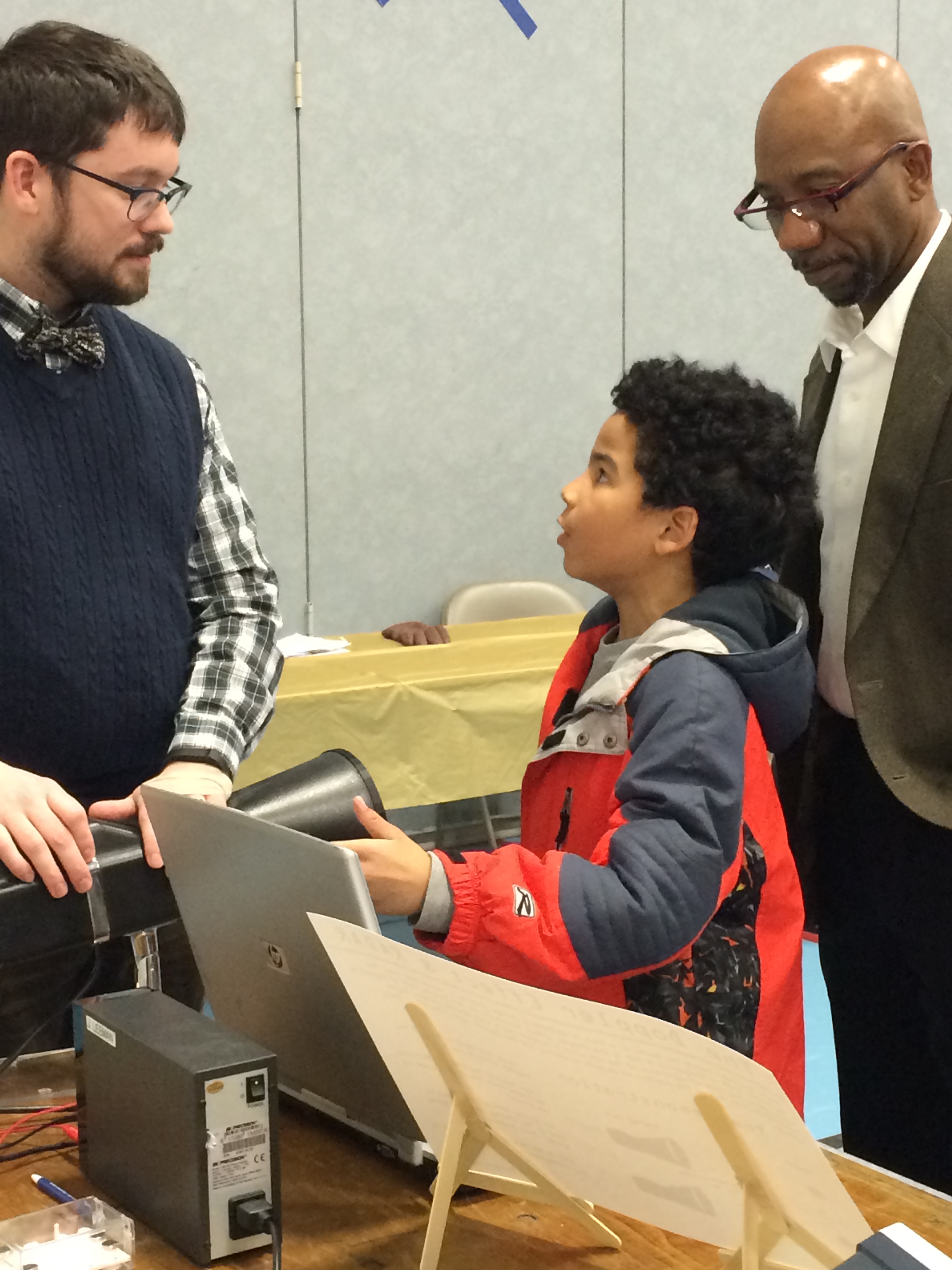
For scientists, communicating with the public can be difficult. It's easy for us to get holed up in our little niche of work and forget that talking about a topic like power spectra isn't everyday to pretty much everyone. Outreach events like this present a great opportunity to work on those skills! This particular event was especially challenging for me because the children were K-5, much younger than I usually talk to. With high school students you can maybe talk about the frequency of a wave and not get too many lost looks, but not with grade-schoolers!
The other difficulty was adapting what are deep topics (each demo is an entire field of research, or several) to the short attention span we had to work with. Elementary school teachers are masters of this and I would love to get some ideas from them on how to work with the younger minds. I spent most of my time talking about the Doppler effect with the RADAR (it's the topic my lab mates were least comfortable with since we don't deal with RADAR at work generally). By the end of the science fair, I had an explanation down that involved asking the kids to wave their hand slowly and quickly in front of the RADAR and listen to how the pitch of the output changed. Comparing that to the classic example of the pitch bending of a passing fire truck siren seemed to work pretty well. I had a "waterfall" spectra display that showed the measured velocity with time, but other than trying to get the line to go higher than their friends, it didn't get much science across (though lots of healthy competition and physical exercise was encouraged).
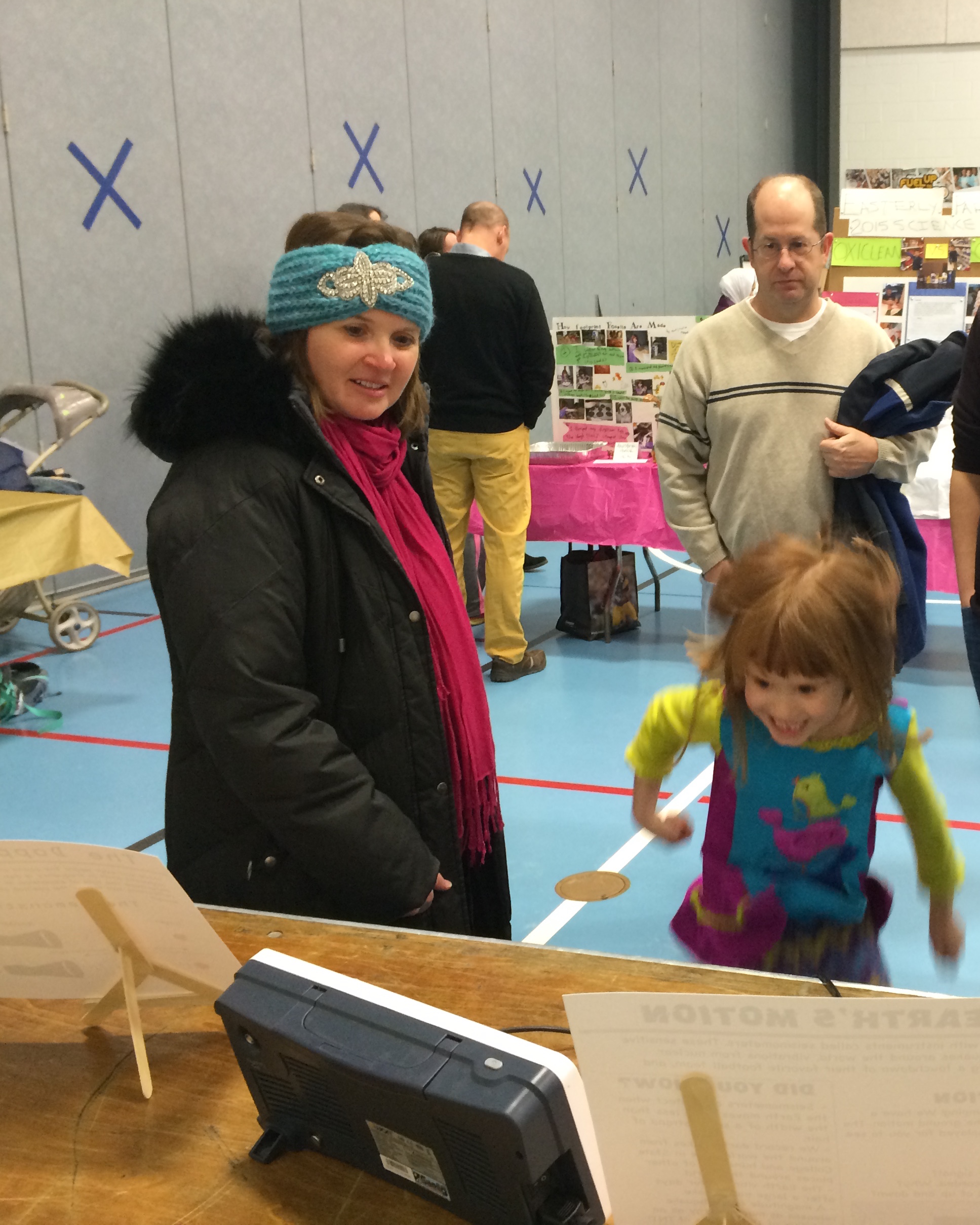
An excited student jumps up and down to see herself on a geophone display.
In the past, I've pointed out the value of being an "expert generalist". All of us were tested in any possible facet of science by questions from the kids and their parents. I ended up discussing gravitational sling-shot effects on space probes with a student and his parents who were incredibly interested in spaceflight. I also got quizzed about why the snow forecasts had been so bad lately, when the next big earthquake would be, and a myriad of other questions. Before talking to any public group, it's also good to make sure you are relatively up-to-date on current events, general theory, and are ready to critically think about questions that sound deceptively simple!
The last point I want to bring up today is the idea of comparisons. These are numbers that one of my committee members likes to say he "carries around in his shirt pocket." These are numbers that let us, as scientists, relate to others that are non-specialists and give us some physical attachment to a measurement. What do I mean? Let's say that I tell you that tectonic plates move anywhere from 2-15 cm/year. Great, first, since we are in the U.S.A., everyone will hold out their fingers to try to get an idea of what this means in imperial units.... not quite 1-6 in/year. That's better, but a year is a long time and I can't really visualize moving that slowly since nothing I'm used to seeing everyday is that slow... or is it? Turns out that fingernails, on average, grow 3.6 cm/year and hair grows about 15 cm/year. Close enough! In Earth science we have lots of approximate numbers, so these tiny differences are not really that bad. Now let's revise our statement to the kids to say: "The Earth is made of big blocks of rock called plates. These move around at about the speed your finger nails or hair grow!" Now it is something that anyone can relate to, and next time they clip their nails or get a hair cut, they just might remember something about plate tectonics! It's not about having exact figures in the minds of everyone, it's about providing a hand-hold that anybody can relate to! This deserves a post to itself though.
That's all for now, but I'd love to hear back from anyone who has elementary education experience or has their own "shirt pocket numbers."
I would like to announce the official release of the first episode of the "Don't Panic Geocast!" This is something that has been in the works since earlier this summer. Each week Shannon Dulin and I will be discussing geoscience (geology, meteorology, etc) and technology. Please be sure to add us to your feeds and checkout our first show!
This year at the fall meeting of the American Geophysical Union, I presented an education abstract in addition to my normal science content. In this talk, I wanted to raise the awareness of how easy it is to work with electronics and collect geoscience relevant data. This post is here to provide anyone that was at the talk, or anyone interested, with the content, links, and resources!
Sensors and microcontrollers and coming down in price thanks to mass production and advances in process technology. This means that it is now incredibly cheap to collect both education and research grade data. Combine this with the emergence of the "Internet of Things" (IoT), and it makes an ideal setup for educators and scientists. To demonstrate this, we setup a small three-axis magnetometer to measure the Earth's magnetic field and connected it to the internet through data.sparkfun.com. I really think that involving students in the data collection process is important. Not only do they realize that instruments aren't black boxes, that errors are real, and that data is messy, but they become attached to the data. When a student collects the data themselves, they are much more likely to explore and be involved with it than if the instructor hands them a "pre-built" data set.
For more information, watch the 5-minute talk (screencast below) and checkout the links is the resources section. As always, email, comments, etc are welcome and encouraged!
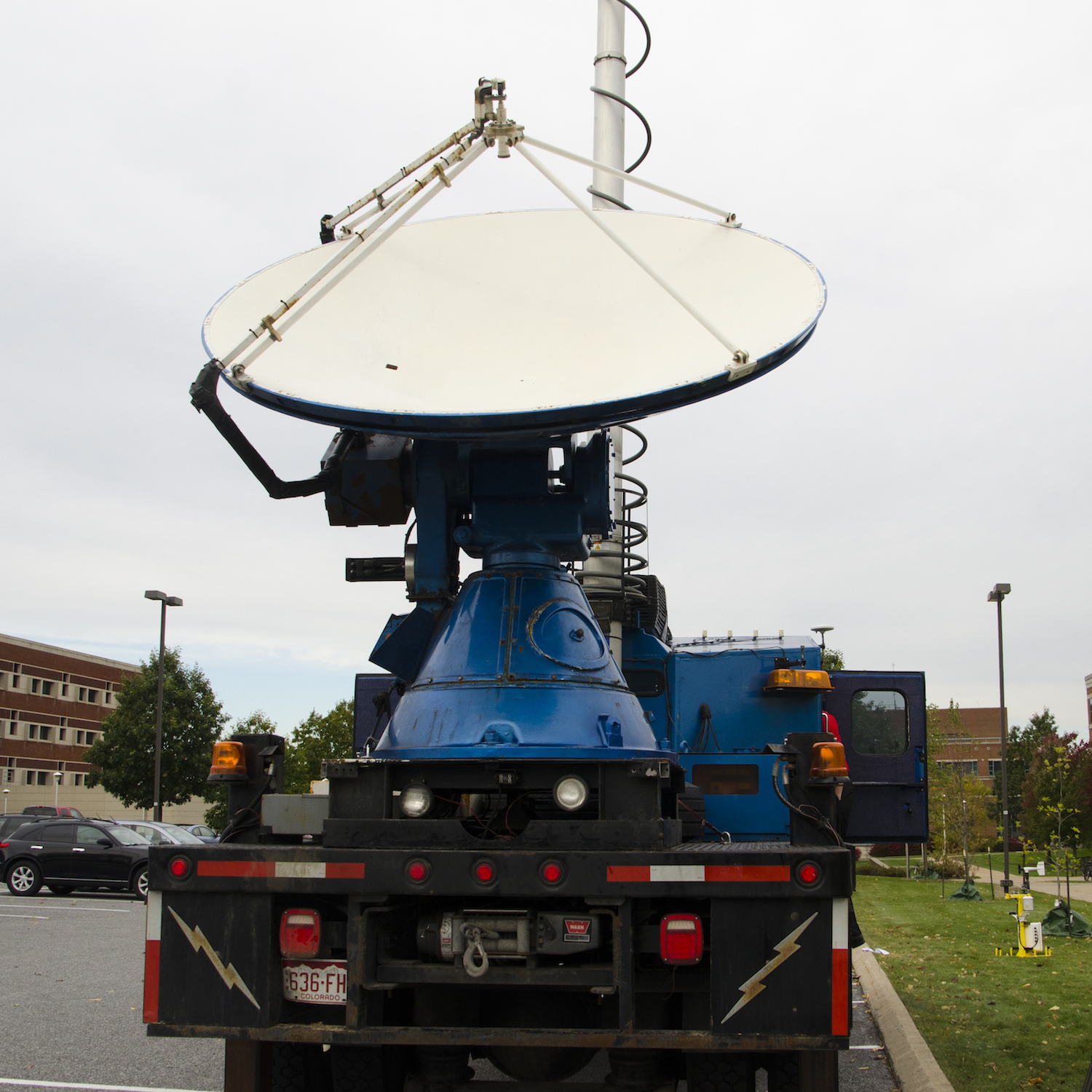
Recently, Penn State was lucky enough to have the "Doppler on Wheels" or DOW visit for two weeks through an NSF education grant! The truck, owned and operated by the Center for Severe Weather Research, is probably familiar to you if you have watched any of the storm chasing television shows or are interested in severe storms. Dr. Yvette Richardson and Dr. Matt Kumjian were the faculty hosts and incorporated the radar into classes they are teaching.
I've always believed in getting students involved with data collection. If students collect the data, they are attached to it and begin to see the entire scientific process. Data doesn't just appear, real data is collected, often with complex instruments, and processed to remove various problems, corrections, etc. It's not everyday that students get to collect data with a state-of-the-art radar though!
For this entry we're going to try a video format again. Everyone seemed to like the last video entry (Are Rocks like Springs?). Keep the feedback coming! It was a bit windy, but I've done what I can with the audio processing. A big thanks to everyone who let me talk with them! As always, keep updated on what's happening by following me on twitter (@geo_leeman). This week I'll be off to New York to hear Edward Tufte talk about data visualization, so expect updates about that!