This morning there was a magnitude 7.1 earthquake beneath Alaska. Alaska is no stranger to earthquakes, and I'm not going to talk about the tectonics, but I wanted to share the ground motion videos I produced for the event. Also be sure to checkout the ground motion videos over at IRIS as well. At present no major damage or injury was reported. Though CNN did sensationalize the earthquake (as they always do):
First a video from a nearby station, Homer, AK. About 8 mm maximum ground displacement with some pretty large ground accelerations.
The earthquake recorded in Australia. Not as exciting, but notice the packets of waves towards the end of the video, these are the surface waves that took the longer route around the globe compared to their earlier counter parts. (Called R1/R2 and G1/G2.)
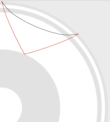
Here's a central US station near where I grew up. Nice surface waves and a good example of what looks like the PcP phase (P-wave reflected off the outer core of the planet.) The PcP phase is at about 604 seconds, around 100 seconds after the P wave. In the figure below the movie, the approximate PcP path is red, the P path is black. Pretty neat!
It is finally summer and I see lots of people playing all sorts of outdoor sports. While I have never been a big sports player, it is fun to watch. There are a lot of physics involved in most sports, so maybe that is a line of posts worth investigating. I do have a post series on open source science planned that will last most of the summer, but maybe we can keep sports in mind next year?
This post is a resurrection of a post I started a couple of years ago and never got around to finishing. In an effort to tie up loose ends, here we go! How does a frisbee fly? I wondered this when we discovered that my fiancée can throw a frisbee upside down sometimes with results that flew surprisingly far. To understand what is happening we need to look at the fundamental physics of frisbee flight, make some measurements, then try to draw some conclusions. Turns out there is a lot of research on the aerodynamics of flying discs, so I'll hit the important points and leave links to let you dig down the wiki-hole with me if you wish. To start out, check out a copy of "Spinning Flight" by Ralph Lorenz at your library.
The physics of frisbee flight
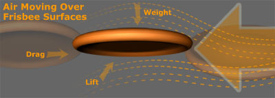
While in flight, our frisbee will experience several forces governing its movement including gravity, lift, drag, and a torque from its angular momentum. We will quickly look at each of these, but we are not going to fully model the system (though it could be fun!)
Forces on a frisbee. (Image: illumin.usc.edu)
First off, Gravity is the most obvious and intuitive of these forces. Everything is pulled towards the earth's center of mass by gravity at about 9.81m/s/s. If we just place the frisbee on the table, it will experience a force resulting from the acceleration of gravity. If we drop it, it will be accelerated downward. The velocity of falling objects has been fully investigated and we won't go into that too deeply. For now, simply assume that we could calculate the velocity of a dropped object or calculate the acceleration of an object if we know its fall rate.
Lift is what may be the most important force in this study. Believe it or not, a frisbee experiences lift following the same principles as a traditional wing or rotor blade. As the frisbee cuts through the air, some of the oncoming air goes over the frisbee, some goes under. The air streams have to meet up in the lee of the frisbee and since we cannot create or destroy air, we must have continuity and conservation. The air on top has to move faster for this to hold, it has longer to travel after all, and the air below can move more slowly. Thanks to Bernoulli's principle, we know that air moving faster will have a decreased pressure. This isn't anything new; in fact, Daniel Bernoulli published this idea in 1738! With fast air on top of the frisbee and slower air below, there is high pressure below and low pressure above the disk. From a difference in pressure we get the force of lift (more generally called a pressure gradient force).
Lift force from a pressure differential. (Image web.wellington.org)
Drag is the reason that our frisbee does not fly off into the distance. Drag is the force that slows the frisbee down as it pushes through the dense atmosphere. We could try to measure the drag through our later analysis, but that itself it a very deep task that we could spend a lot of time on.
Finally, comes the torque from the angular momentum of our frisbee. Have you tried to throw a frisbee without spinning it? In theory it would fly right? It's just a circular wing after all. Well, that turns out to be a pretty unstable way to fly your disc. Generally it will turn up, stall, and then fall like a rock. Why? Thanks to some spatial change in the lift force, the front of the disc will be lifted with slightly more force than the back, causing the disc to torque over to the back. In fact, I'll save you the trouble, you can watch my feeble attempts below. We could try to outfit our frisbee with control surfaces to help it maintain the proper angle of attack, but that is heavy, complicated, and would mean dead batteries would plague playing kids and dogs. Surely there is a more simple way?
Of course! Let's spin the frisbee when we throw it! When we throw the disc and it spins, we get gyroscopic stability and the possibility to see the cool spinning designs we print on the toy. We can determine that this torque will point vertically through the top of the frisbee. If you remember the right hand rule, you'll see that for my right-handed clockwise throw, the torque vector will point towards the ground. For the south-paws out there, your torque vector will point towards the sky. The important thing is that it will try to counteract the tendency of the lift moment to make the frisbee backflip. Granted, it will not win forever. Eventually the flight will become unstable, but we can maintain steady flight for several seconds. Depending on the force balance, we'll also expect to see the frisbee's vertical axis precess around true "up".
Taking measurements
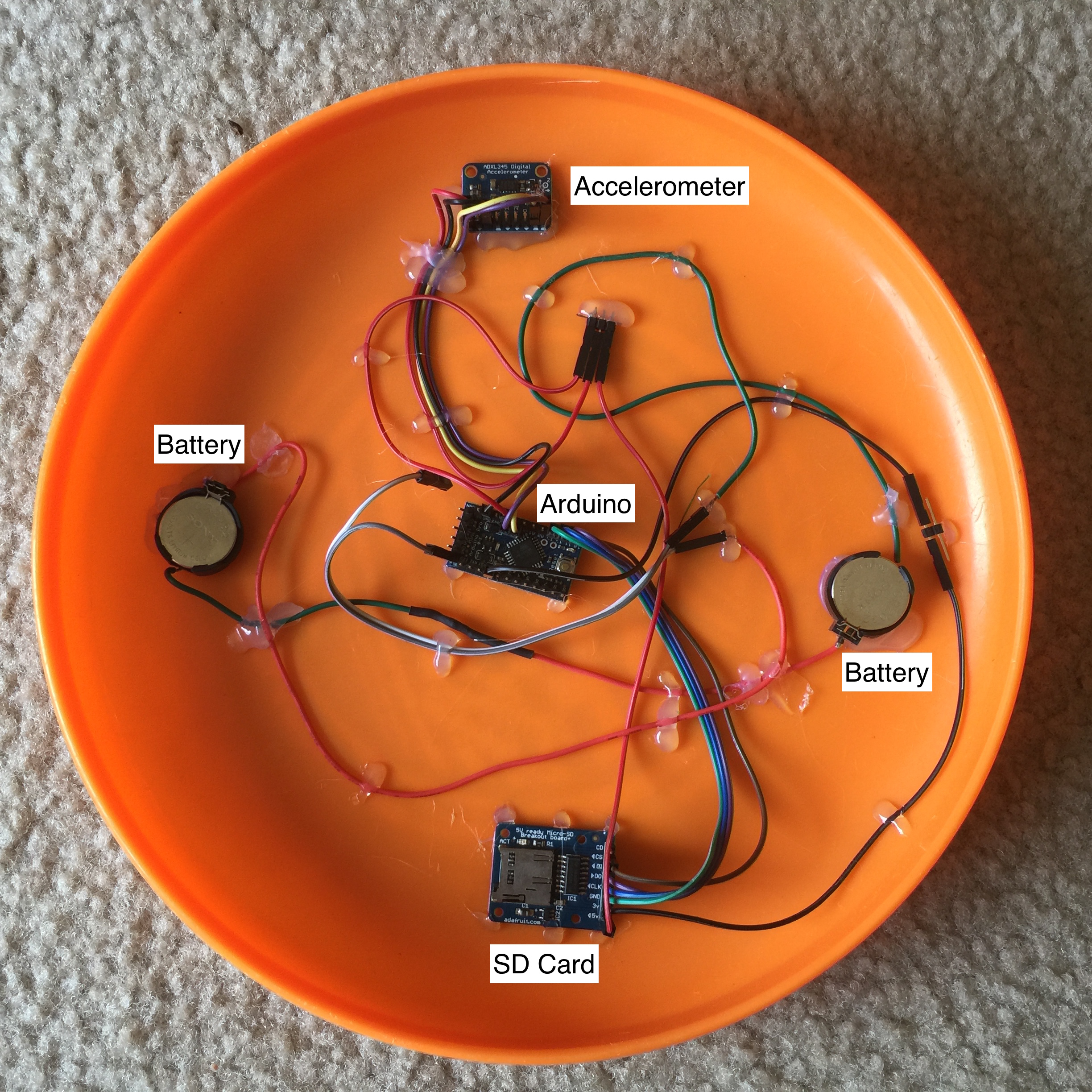
To take some measurements of frisbee flight, I created an instrumented frisbee. Turns out, I'm not the first one to do this. Lorenz made an instrumented frisbee in the early 2000's and then improved it by adding a plethorera of sensors. I decided that a simple accelerometer would be enough for my investigation. While adding angle sensors and such would be interesting, let's keep it simple for a first pass. Maybe adding a 9 degree of freedom inertial measurement unit would be fun, but that's an idea for another time. Actually, the gyroscope data from that would be incredibly useful.
I used an Arduino Pro Mini for my micro controller, an accelerometer, and SD card logger for the sensor and logging system. I ended up just trying to read the sensor in single shot mode as fast as possible. This gave a data rate of around 180-200 Hz with time-stamps in microseconds on each packet. Sure, we could make this part a little more slick, but again, the KISS principle rules for these first hacks at a problem . Power comes from a pair of CR2032 coin cell batteries. All of this was hot glued down and hopefully made as aerodynamic as possible without coweling the whole assembly. Should we wish to improve this, I would directly solder the wires to the boards instead of using header connectors and cover everything in kapton tape.
If you are interested in trying this yourself, the Arduino sketch is at the bottom of this post.
To approximate the speed of the frisbee I will have some video of the flights that we can look at to get some rough numbers to work with. These were just filmed with a DSLR camera, so this is something you can try at home! The newer iPhones are actually even faster than this camera, but I didn't have a tripod mount handy for my 6+ when I filmed this.
Data analysis
First, let's look at the film of a flight to figure out how fast the frisbee throw is on average. We could look at how long the flight was and how far is was and get an average velocity with v=d/t. That's great, but we can do one better! Through the magic of image tracking, we can get the position of the frisbee in each frame of the video and calculate the velocity profile during the flight. While probably not totally necessary, why not?
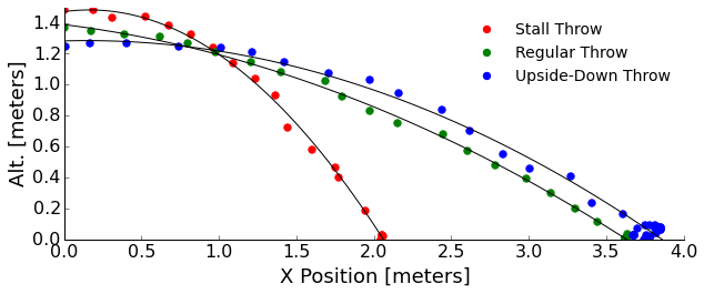
I'll use the Tracker video analysis software for this. We read in the video, setup some coordinate systems, markers, etc, and let it churn. If the frisbee veers in the third dimension (into or out of the screen) we won't get that information because we are just tracking its center in a 2D picture. Hence, I'll try to keep the throws gentle! We'll look at the stall, upside-down, and normal throws:
To keep this short, I'll tell you that the forward speed of these throws looks to top out at about 5 m/s. Again, we could go down the hole of getting drag from the slight deceleration in forward speed with time, but it really doesn't slow us much... the ground beats drag to stopping our frisbee.
We can see that the stall throw drops very quickly without really flying. In fact, it mostly is flipping end-over-end. The regular and upside-down throws look like they have a similar flight profile from the video. This means I must have not been as consistent as I had hoped with my throwing strength. We know that without the lift component that the upside-down throw should follow a more parabolic path than the regular throw. Also, my regular throw was pretty weak to keep the frisbee in the frame and minimally veering, so it didn't have enough lift to show us long periods of stable flight.
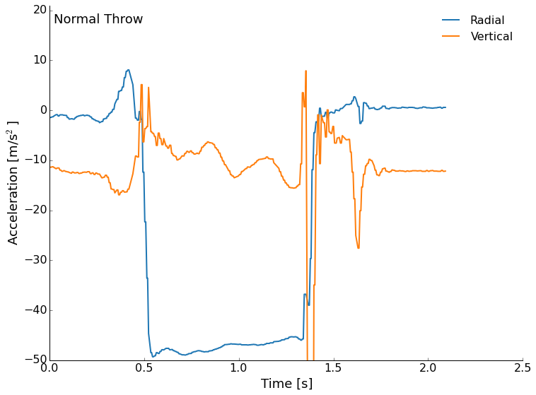
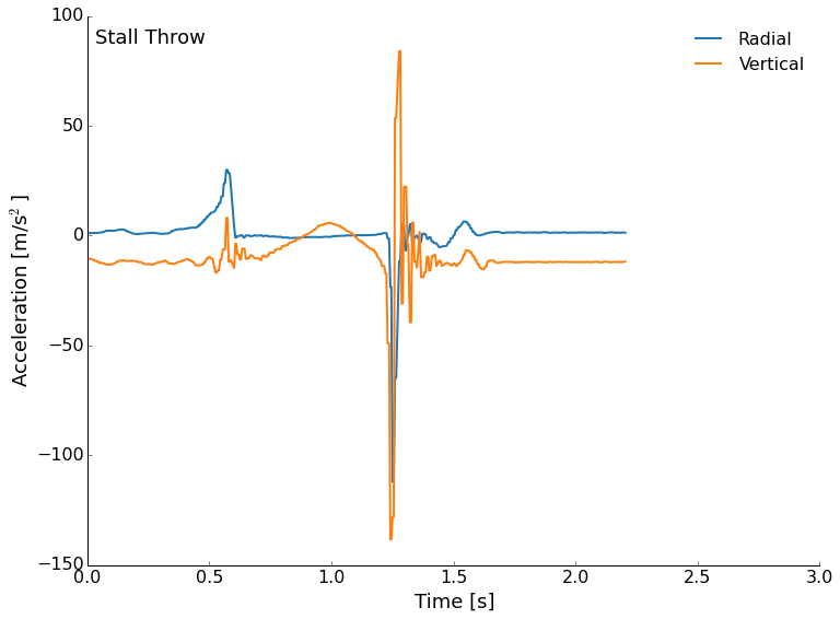
Next, let's look at the accelerometer data. The data is stored in a text file with the millisecond time stamp, and then each of the three axes acceleration measurements. I've plotted the radial (outward from the center) and vertical accelerations. Since the accelerometer was mounted near the rim of the frisbee, we will see relatively large signals from the wobble in flight.
We'll start with the normal throw this time. The accelerometer is roughly calibrated at the factory, but don't worry about the absolute values too much here. We see me pull back to throw as a upturn in the radial, then a large negative (outward) acceleration from the spinning of the disc during flight. Roughly a couple of g's here. The vertical is interesting through. We see the roughly -10m/s/s from the Earth's gravity as a prepare to throw and after the landing, but during flight we see a near zero vertical acceleration that trends downward. What is it? Lift! This is the flight of the frisbee that is gradually reduced as drag slows us and the angle of attack becomes non-ideal. We are expecting that we don't totally counteract gravity because flight is not sustained and our frisbee does not go on forever. This was a pretty gentle and short flight, but followed our expectations in terms of the forces at work. We can even see some precession in the vertical in the neighborhood of about 4 times/second.
Next, we'll look at the stall throw. This isn't spinning so we don't expect to see a lot of radial acceleration once the throw leaves our hands, but we do expect to see some lift for a short period of time, then a stall and fall. That is what we get, too! The spike in the blue curve at 0.5 seconds is my push to accelerate the frisbee, then there are few other radial accelerations recorded (except the impact). There should be some small accelerations from the flip of the disc, but they are tiny here. The vertical trend up and down just before 1 second is the frisbee flipping over once. The only real lift is just a tiny fraction of a second before the front is lifted up. After that, we are really just in free-fall.
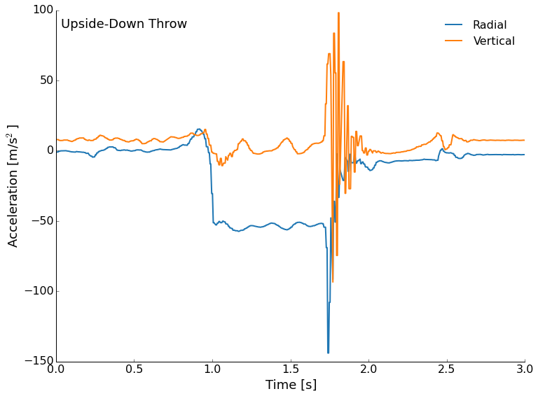
Finally, the elusive upside-down throw. The frisbee starts out upside-down, so the acceleration of gravity now shows as positive (look after the landing for example). We still see radial acceleration from the spinning and we also see a reduction in the vertical acceleration. This can't be lift, but is probably some axis mis-alignment on the sensor. We still see precession as the torque tries to keep the disc horizontal.
What did we learn?
We learned about all of the forces at play in the flight of a frisbee, lift, drag, etc. We measured some flight paths and acceleration profiles. These were not quite as clear cut as I had hoped though. We still saw that flying right side up works pretty well, but upside down "flight" is basically spin-stabilized falling with a lot of forward momentum. Throwing with no spin quickly results in a pitch-up and stall.
We'll see what happens with this. If people are interested we could think about adding an IMU to the setup with better positioning and balance. We could also just put a light on a frisbee and track it with a time-lapse photo. This turned out to be a fascinating look at flight, acceleration measurement, and video tracking! If you are wondering about numerical modeling, there is a really nice report from MIT that develops a good model.
#include <SPI.h>
#include <SD.h>
#include <Wire.h>
#include <Adafruit_Sensor.h>
#include <Adafruit_ADXL345_U.h>

/* Assign a unique ID to this sensor at the same time */
Adafruit_ADXL345_Unified accel = Adafruit_ADXL345_Unified(12345);

const int chipSelect = 4;

File dataFile;

void displaySensorDetails(void)
{
sensor_t sensor;
accel.getSensor(&sensor);
Serial.println("------------------------------------");
Serial.print ("Sensor: "); Serial.println(sensor.name);
Serial.print ("Driver Ver: "); Serial.println(sensor.version);
Serial.print ("Unique ID: "); Serial.println(sensor.sensor_id);
Serial.print ("Max Value: "); Serial.print(sensor.max_value); Serial.println(" m/s^2");
Serial.print ("Min Value: "); Serial.print(sensor.min_value); Serial.println(" m/s^2");
Serial.print ("Resolution: "); Serial.print(sensor.resolution); Serial.println(" m/s^2");
Serial.println("------------------------------------");
Serial.println("");
delay(500);
}

void displayDataRate(void)
{
Serial.print ("Data Rate: ");

switch(accel.getDataRate())
{
case ADXL345_DATARATE_3200_HZ:
Serial.print ("3200 ");
break;
case ADXL345_DATARATE_1600_HZ:
Serial.print ("1600 ");
break;
case ADXL345_DATARATE_800_HZ:
Serial.print ("800 ");
break;
case ADXL345_DATARATE_400_HZ:
Serial.print ("400 ");
break;
case ADXL345_DATARATE_200_HZ:
Serial.print ("200 ");
break;
case ADXL345_DATARATE_100_HZ:
Serial.print ("100 ");
break;
case ADXL345_DATARATE_50_HZ:
Serial.print ("50 ");
break;
case ADXL345_DATARATE_25_HZ:
Serial.print ("25 ");
break;
case ADXL345_DATARATE_12_5_HZ:
Serial.print ("12.5 ");
break;
case ADXL345_DATARATE_6_25HZ:
Serial.print ("6.25 ");
break;
case ADXL345_DATARATE_3_13_HZ:
Serial.print ("3.13 ");
break;
case ADXL345_DATARATE_1_56_HZ:
Serial.print ("1.56 ");
break;
case ADXL345_DATARATE_0_78_HZ:
Serial.print ("0.78 ");
break;
case ADXL345_DATARATE_0_39_HZ:
Serial.print ("0.39 ");
break;
case ADXL345_DATARATE_0_20_HZ:
Serial.print ("0.20 ");
break;
case ADXL345_DATARATE_0_10_HZ:
Serial.print ("0.10 ");
break;
default:
Serial.print ("???? ");
break;
}
Serial.println(" Hz");
}

void setup(void)
{
Serial.begin(9600);
Serial.println("Accelerometer Test"); Serial.println("");

/* Initialise the sensor */
if(!accel.begin())
{
/* There was a problem detecting the ADXL345 ... check your connections */
Serial.println("Ooops, no ADXL345 detected ... Check your wiring!");
while(1);
}

/* Set the range to whatever is appropriate for your project */
accel.setRange(ADXL345_RANGE_16_G);
// displaySetRange(ADXL345_RANGE_8_G);
//accel.setRange(ADXL345_RANGE_4_G);
// displaySetRange(ADXL345_RANGE_2_G);

/* Display some basic information on this sensor */
displaySensorDetails();

/* Display additional settings (outside the scope of sensor_t) */
displayDataRate();
//displayRange();
Serial.println("");
Serial.print("Initializing SD card...");
// make sure that the default chip select pin is set to
// output, even if you don't use it:
pinMode(SS, OUTPUT);

// see if the card is present and can be initialized:
if (!SD.begin(chipSelect)) {
Serial.println("Card failed, or not present");
// don't do anything more:
while (1) ;
}
Serial.println("card initialized.");

char filename[15];
strcpy(filename, "ACCLOG00.TXT");
for (uint8_t i = 0; i < 100; i++) {
filename[6] = '0' + i/10;
filename[7] = '0' + i%10;
// create if does not exist, do not open existing, write, sync after write
if (! SD.exists(filename)) {
break;
}
}

dataFile = SD.open(filename, FILE_WRITE);
if( ! dataFile ) {
Serial.print("Couldnt create ");
Serial.println(filename);
while(1);
}
Serial.print("Writing to ");
Serial.println(filename);
}

void loop(void)
{
/* Get a new sensor event */
for(int i=0; i < 100; i++){
sensors_event_t event;
accel.getEvent(&event);
dataFile.print(millis());
dataFile.print(",");
//log_float(event.acceleration.x,999,8,5);
dataFile.print(event.acceleration.x,5);
dataFile.print(",");
//log_float(event.acceleration.x,999,8,5);
dataFile.print(event.acceleration.y,5);
dataFile.print(",");
//log_float(event.acceleration.x,999,8,5);
dataFile.print(event.acceleration.z,5);
dataFile.println("");
}
dataFile.flush();
}
Over the last few months construction crews have been hard a work tearing into the building adjacent to mine on the Penn State campus. Lots of demolition has been happening as the old building is completely cleaned out and being rebuilt. Some of the noise has been so strong that we could feel it next-door. As a data-nut, my first thought was "I'm going to look at this on our seismometer!"
At the base of Deike building (the geoscience building), we have a seismometer. The station, WRPS "We aRe Penn State", has been in operation on an isolated pier for some time, so we have lots of data to look at! For our purposes, I downloaded the entire month of October for 2013 and 2014. There are some hours/days that are missing, but we'll ignore those and work with what we have. This is a common problem in geoscience!
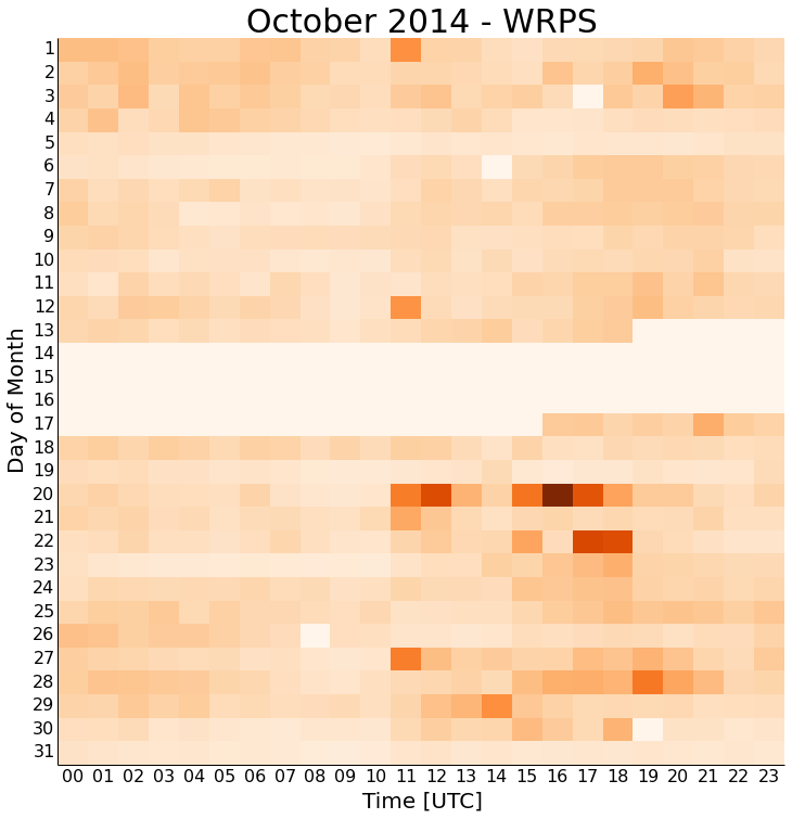
First let's just make a plot of this year's data. Each square represents one hour (24 squares in a row), and each row represents one day. Missing data is the lightest shade. The squares are colored by the strength of the seismic energy received during that hour; the darker the square, the more energy received.
You'll immediately notice that there is always more noise starting about 11 UTC, which is the 7-8 AM hour locally. This is about when people are coming into work, vibrating the ground and buildings on campus as they do. The noise again seems to die off about 21 UTC or the 5-6 PM hour locally. This again makes sense with people leaving work and school. This isn't split finely enough to look for class change times on campus, but that could always be another project.
The other thing to point out is the dates of October 4-5,11-12,18-19,25-26. These are the weekends! You notice there is less of the normal daily noise traffic with fewer people on campus and construction halted. There is a repeating noise event at 11 UTC on the 1st, 12th, 20th, and 27th. I'm not sure what that is yet, but looking at more months of data may indicate if that event is associated with equipment starting up, or is really random.
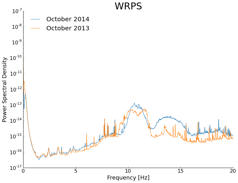
While these daily life trends are interesting, they have been observed before. This whole discussion started with construction and how it was affecting the noise we saw on our local station. To examine this, I made a stacked power spectral density plot. Basically, this shows us how much energy is recorded at different frequencies. The higher frequencies would be human activity.
We can see that the curves from 2013 and 2014 are very similar, with the exception of the 11-16 Hz range. In that range, the energy is higher in 2014 than in 2013 without construction by about a factor of 10. That range makes sense with construction activity as well! The energy remains elevated even after the main bump out to 20 Hz.
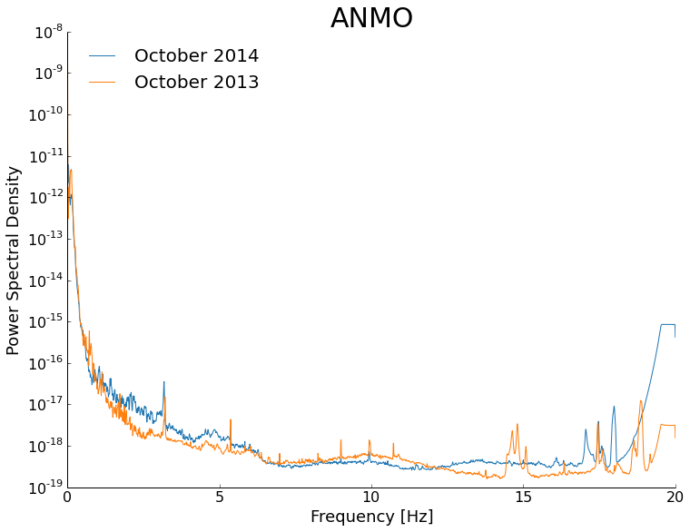
You might be thinking that such a bump could be due to anything. That's not necessarily true considering that we have stacked a month's worth of data for each curve. To show how remarkably reproducible these curves are, I made the same plot for the same times with a station in Albuquerque, New Mexico.
In the Albuquerque plot, the two years are very similar, nothing like the full order of magnitude difference we saw in University Park. There are obviously some processing effects near 20Hz, but those are not actual signal differences, just artifacts of being near the corner frequency.
That's it for now! If there is interest, we can keep digging and look at signals resulting from touchdowns in football games, class changes, factories, etc. A big thank you to Professor Chuck Ammon as well for lots of discussion about these data and processing techniques.
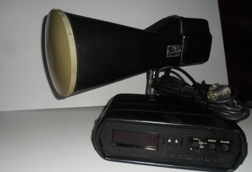
When you hear "radar", you probably think of weather radar and a policeman writing a ticket. In reality there are many kinds of radar used for everything from detecting when to open automatic doors at shops to imaging cracks in concrete foundations. I've always found radar and radar data fascinating. Some time back I saw Dr. Gregory Charvat modify an old police radaron YouTube and look at the resulting signal. I happened to see that model of radar (a 1970's Kustom Electronics) go by on EBay and managed to buy it. I'm going to present several experiments with the radar over a few posts. If you want to learn more about radar and the different types of radar I highly recommend Dr. Charvat's book Small and Short-Range Radar Systems. I haven't bought a personal copy yet, but did manage to read a few chapters of a borrowed copy.
The doppler radar I purchased. I'm not using the head unit.
The radar I have outputs the doppler shift of a signal that is transmitted, reflected, and received. Doppler is familiar to all of us as we hear the tone of a train horn or ambulance change as it rushes past us. Since there is relative motion of the transmitter (horn) and receiver (your ears), there is a shift in received frequency. Let's say that the source emits sound at a constant number of cycles per second (frequency). Now let's suppose that the distance between you and the source begins to close quickly as you move towards each other. The apparent frequency will go up because the source is closer to you each emitted cycle and you are closer to the source!
The doppler effect of a moving source. Image: Wikipedia
This particular radar transmits a signal at a frequency of 10.25 GHz. This outgoing signal is continually transmitted and reflected/scattered off of objects in the environment. If the object isn't moving, the signal returns to the radar at 10.25 GHz. If the object is moving, the signal experiences a doppler shift and the returned frequency is higher or lower than 10.25 GHz (depending on the direction of travel). This particular radar can be easily hacked and we can record the doppler frequency out of a device called a mixer. The way this unit is designed, we can't tell if the frequency went up or down, just how much it changed. This means we don't know if the targets (cars) are coming or going, just how fast they are traveling. Maybe in a future set of posts, we'll build a more complex radar system such as the MIT Cantenna Radar. Be sure to comment if that's something you are interested in.
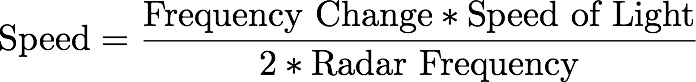
Since we'll be measuring speeds that are "slow" compared to the speed of light, we can ignore relativistic effects and calculate the speed of the object knowing the frequency change from the mixer, and the frequency of the radar.
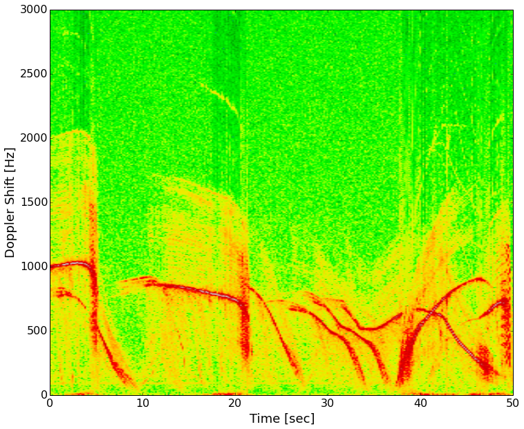
I took the radar out to the street and recorded several minutes of traffic going by, including city busses. Making a plot of the data with time increasing as you travel left to right and doppler frequency (speed) increasing bottom to top, we get what's known as a spectrogram. Color represents the intensity of the signal at a given frequency at a certain point in time.
Speeds of several cars on my street. 1000 Hz is about 33 mph and 500 Hz is about 16 mph.
The red lines are strong reflectors (the cars). Most of the vehicles slow down and turn on a side street in front of the radar. About 30 seconds in there are three vehicles, two slow down and turn, the third again accelerates on past. Next I'll be lining up a video of these cars passing the radar with the data and you'll be able to hear the doppler signal. To do that I'm learning how to use a video processing package (OpenCV) with Python.
In the next few installments, we'll look at videos synced with these data, radar signatures of people running, how radar works when used from a moving car, and any other good targets that you suggest!