What's the most complicated way to say it's raining? Well, if you know me, you know it will involve electronics, sensors, and signal processing! This post was originally going to compare the fall velocity for rain, sleet, and snow. Unfortunately, I haven't been lucky enough to be home to run my radar when it was snowing. It will happen this winter, but we'll start looking at some data now. Want to review radar before we get started? We have already talked about looking at the doppler signature of cars and got a tour of a mobile weather radar.
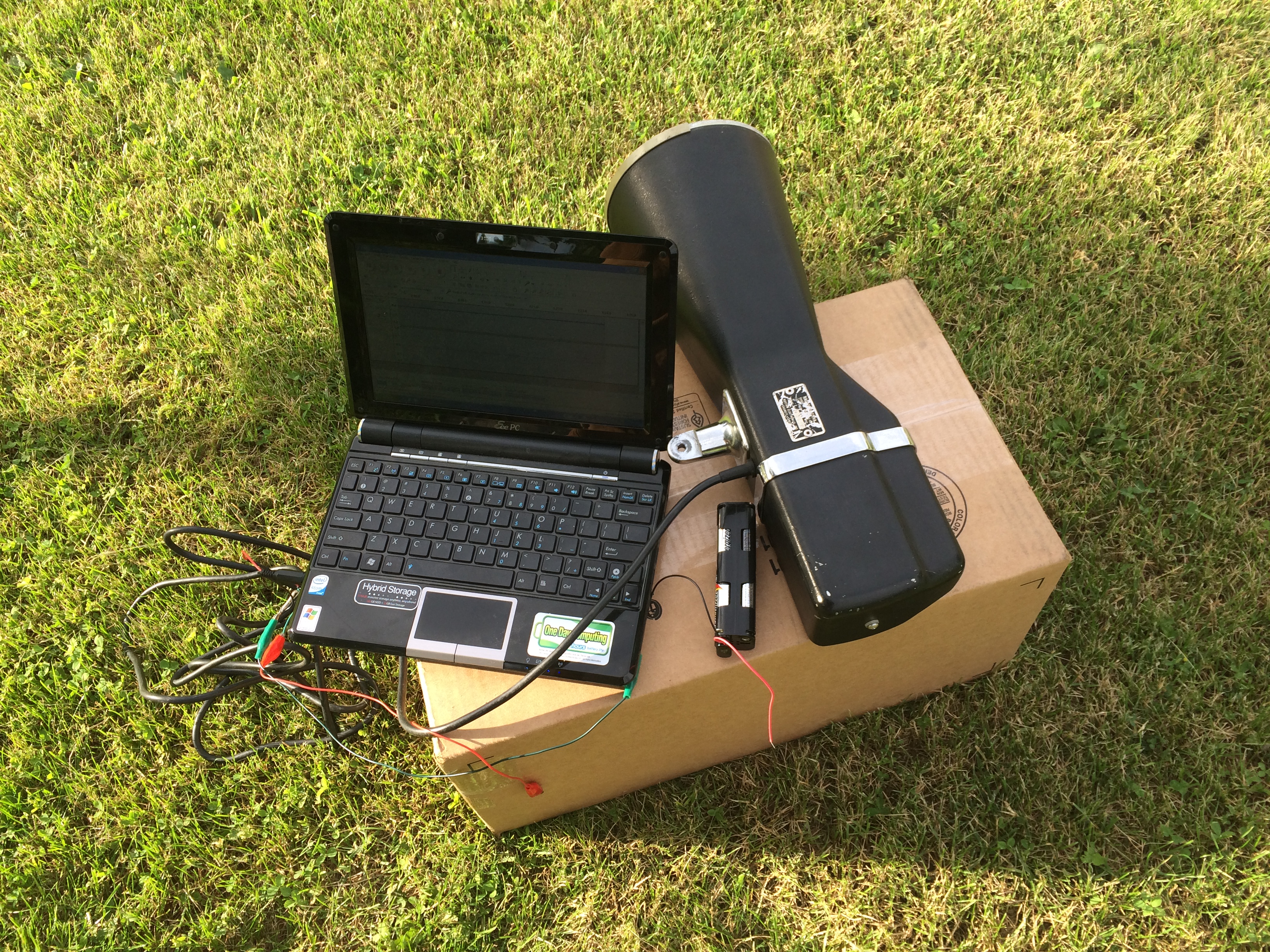
Back in October we had a couple of squall lines come through. On the 3rd, there was a significant event with two lines of storms. I had just been experimenting with measuring rainfall velocity with the modified X-band radar, so I decided to try another experiment. I put the radar unit in a trashcan and covered it with plastic bags. Then I sat it outside on our balcony and recorded for about 2.5 hours.
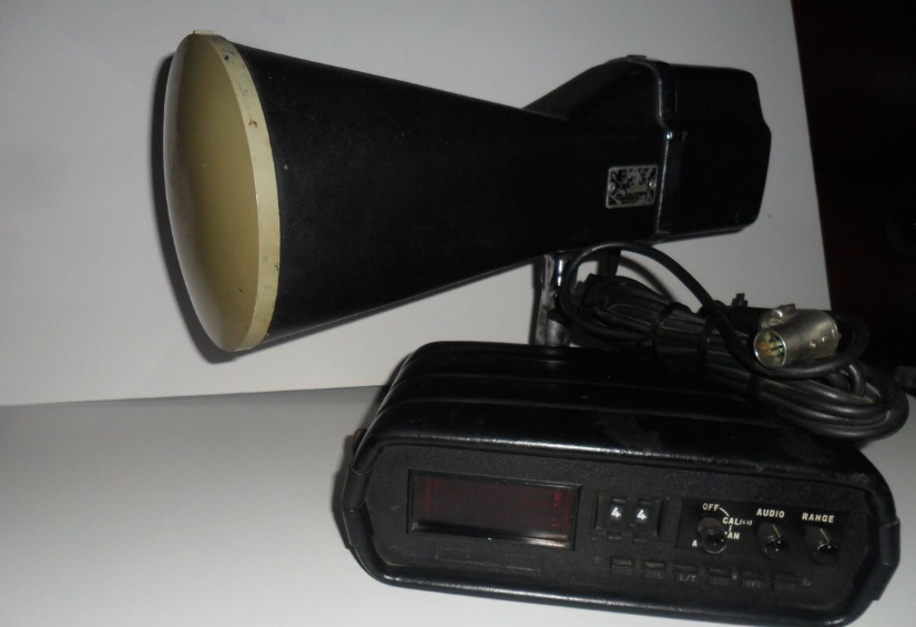
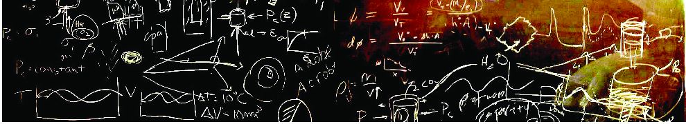
Testing the radar setup before the rain with some passing cars as targets.
There is a radar in there! My make-shift rain proof radome. The only problem was a slight heat buildup after several hours of continuous operation.
Not only do we get the doppler shift (i.e. velocity of the raindrops), but we get the reflected power. I'm not going to worry about calibrating this, but we can confidently say that the more (or larger) raindrops that are in the field of view of the radar, the more power will be reflected back.
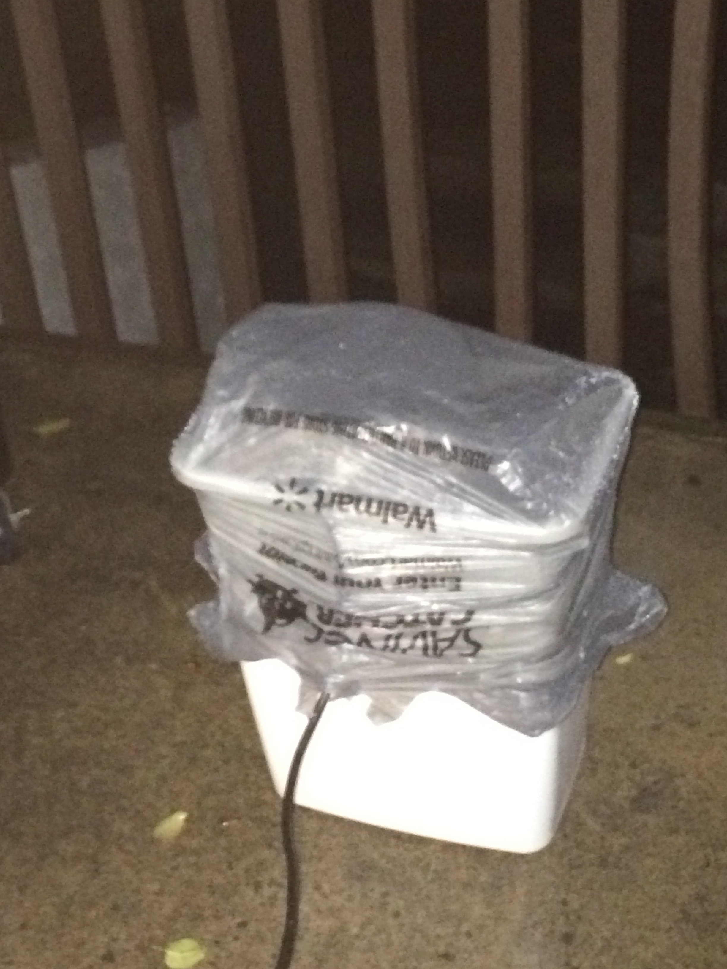
First, let's look at a screenshot of the local weather service radar. You can see my location (blue cross) right in front of the second line of showers. At this point we had already experienced one period of heavy rain and were about to experience another that would gradually taper off into a very light shower. This was one of the nicer systems that came through our area this fall.
A capture of our local weather radar, my location is the blue cross directly ahead of the storm.
Now if we look at the returned power to the radar over time, we can extract some information. First off, I grouped the data into 30-second bins, so we calculate the average returned power twice per minute. Because of some 32-bit funny business in the computations, I just took the absolute value of the signal from the radar mixer, binned it, and averaged.
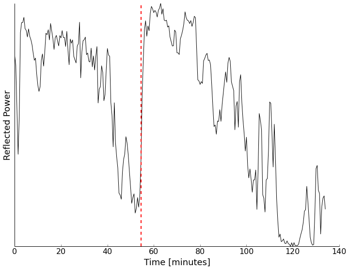
Reflected power received by the radar over time. The vertical red line is the time that the radar screen shot above was taken. We can see the arrival and tapering off of the storms.
From this chart we can clearly see the two lines of storms that came over my location. We also see lots of little variations in the reflected power. To me the rain-rate seemed pretty constant. My best guess is that we are looking at skewing of the data due to wind. This could be solved with a different type of radar, which I do plan to build, but that doesn't help this situation.
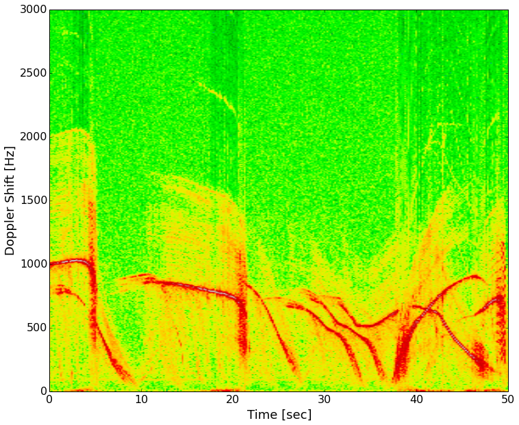
Let's look at what inspired this in the first place, the rainfall velocity. From a chart of terminal velocities, we can see that we expect to get drops falling between 4.03-7.57 m/s for moderate rain and 4.64-8.83 m/s for heavy rain. Taking a 5 minute chunk of data starting at 60 minutes into the data (during high reflectivity on the chart above), we can compute the doppler frequency content of the signal. Doing so results in the plot below, with the velocity ranges above shaded.
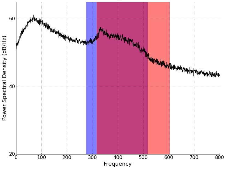
Doppler frequency content of 5-minutes of data starting at 60 minutes into recording. The blue box shows doppler frequencies corresponding to moderate rain, and the red box corresponding to heavy rain.
Based on what I see above, I'd say that we fall right in line with the 0.25"-1" rain/hour data bracket! There is also the broad peak down at just under 100 Hz. This is pretty slow (about 1 m/s). What could it be? I'm not positive, but my best guess is rain splattering and rebounding off the top of my flat radar cap. I'm open to other suggestions though. Maybe part of this could be rain falling of the eve of the building in the edge of the radar view? The intensity seems rather high though. (It was also suggested that this could be a filter or instrument response artifact. Sounds like a clear air calibration may help.)
So, what's next? We'll take some clear-air calibration data and the use data from a Penn State weather station to see what the rain rate actually was and what the winds were doing. Maybe we can get a rain-rate calibration for this radar from our data. See you then!
Thank you to Chuck Ammon for discussions on these data!