Teaching Field Camp Week 2 - Ground Penetrating Radar

Week 2 of camp for the geophysics students was at the new University of Oklahoma Bartell Field Camp. Students were split into three groups and each group rotated through three main geophysical methods: gravity, magnetics, and ground penetrating radar (GPR).  I was responsible for the GPR all week, but we'll briefly discuss everything they did and some problems we had along the way.

Monday the students went on an intro field trip to learn about the geology of the area.  First students walked up the road to 'high camp' noting the sediment basement contact (and what we interpret as a large fault breccia) on the way.  When into the granitic basement there are many mafic dikes, some locations even have dikes crosscut by later intrusions.  The students this year really seemed well prepared to tie the geology into their reports and were very careful in noting/interpreting features.  Next we drove to Tunnel Drive, a short hike that exposes lots of basement deformation and some classic fault examples.  There were also a couple fun stops like Skyline Drive where dinosaur footprints have been preserved as trace fossils.  In the picture below we are looking up at the bottom on an impression likely left by a foot of an ankylosaurus.

The next three days the groups rotated through the geophysical methods.  In this post I'm only going to discuss the GPR collection and data.  The gravity data is currently being processed (so expect a post about it early next week) and the magnetics are posing problems.  Our main magnetometer has an internal problem that prevents us from downloading the data collected.  It is being sent back to the factory and the students will collect new data with an older system next week.  There is also a special magnetic surprise I found in an outcrop that I want to discuss in a more detailed post.

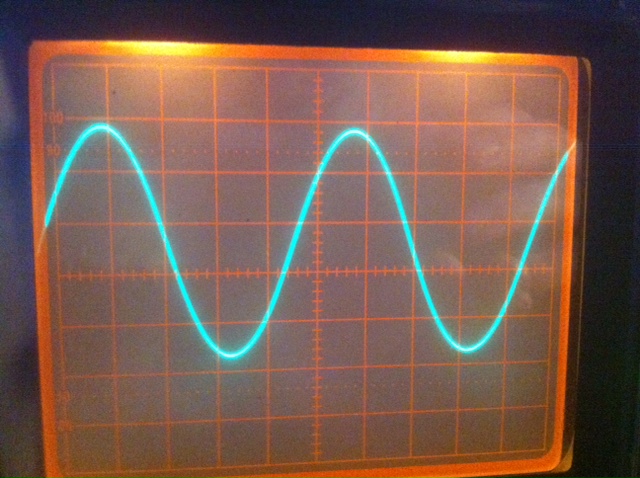
Ground penetrating radar is a technique we haven't really used much recently at OU, but I'm hoping to make a come back with it! The system needed lots of tweaking, adjusting parameters, and fiddling with; after that it obtained some really interesting data.  A ground penetrating radar sends a signal into the rock, which is reflected from various objects/interfaces, so data is interpreted similar to seismic data (only at a different time scale).  Seismic waves travel through rock at around 2200km/second while radar waves are much faster at about 0.1m/nanosecond.  GPR is used extensively in archeology to look for near surface targets and to find bodies during criminal investigations (we have in fact used this system over a mass grave before in Norman... but that's another post all together).

The first day we had students experiment with different parameters over a known target (a metal culvert under a road).  While the target isn't necessarily geologic, we know what it is, where it is, and how big it is.  Using this we setup an ideal parameter set to then examine more interesting geologic features.  Other groups during the week also targeted the culvert for practice, then picked more interesting areas to examine.

First I had to patch together some codes to convert the GPR data from the proprietary DT1 format to a more standard SEGY format.  We then worked up some seismic unix command flows to process that data.  The images shown are not migrated and could benefit from migration, spiking deconvolution, etc.

The first image shown is on the high camp road.  There was a culvert near the surface, but below that are other diffractions from some interesting geological structures.  I'll currently not say any more so students can think about what these are.  The second image shows why this tool could be so valuable.  There was little geology at the surface, but according to the data there is a dipping reflector just under our feet.  What could it be? Maybe with a few more trips up there I'll be able to find it in outcrop somewhere.  There were also some diffractions deeper in this image.  While I do have lots of comments about the GPR parameters, setup, etc I don't think it's so important to discuss.  My goal is to show that there is so much beauty in the complexity of what happened here.  The basement rock is very very old (without an extensive literature search we'll say pre-cambrian, which is ~540 Million years ago).

Friday we took the students on another field trip.  Early in the morning I had to take our other TA, Cullen Hogan, to the airport.  He is leaving us for an internship and will be greatly missed in the last week of the course.  After returning from the Colorado Springs airport the students piled in to drive to one of my favorite views in southern Colorado, Spiral Drive in Salida.  On the way to Salida from Cañon City small sedimentary 'hanging basins' can be found in the mountain sides as we drive through a thrust zone between sediment and basement.  Salida lies in the San Lúis Valley, part of the slow Rio Grande Rift.  The view is always amazing and some complex geology is observed on the way.  Below is a panorama overlooking the collegate peaks I took at this location last year (there wasn't as much snow this time).

Teaching Field Camp Week 1 - Norman, OK

For the next 3.5 weeks I'll be a teaching assistant for the University of Oklahoma geophysics field camp.  The point of the camp is to teach senior geophysics students how field data is collected, processed, interpreted, and applied to the problem.  This is an important capstone class because prior to now students just see geophysical data as equations, numbers, and options in software and on paper.  Now they must hike in the field, observe the geology, collect the data, and finally figure out what it all means.

Week 1 was done in Norman, OK back at the school.  Monday the students listened to lecture on geophysical methods, were introduced to the equipment, and finally were tasked with using differential GPS on the North Oval of campus.  Differential GPS is much more sophisticated than the GPS in your car.  Each unit costs ~$80,000, and one is mounted on a tripod and remains stationary throughout the day.  This station is referred to as the base, and is the most crucial link in any geophysical survey.  The second station is mounted in a backpack and is the rover.  Students walk around with the rover collecting data points, then at the end of the day the base station is used to calibrate the rover data.  We know the base station doesn't move during the day, but it appears to in the data.  This is because GPS locations are highly susceptible to changes in atmospheric humidity, irregularities in the satellite orbits, and a number of other factors.  Without going into more detail, look below at the Excel plot of the oval before and after correction.  Data points are much closer (within centimeters) after correction, and those centimeters make all the difference in some survey environments.  This plot came from one of our students reports that was turned in during the week.

The next objective was to collect a seismic line over a branch of the fault system that slipped during the earthquake sequence of November 2011 in central Oklahoma.  Setting out a seismic line is a long, arduous task, so the students needed a practice day.  We setup a short (~300m) line by the school's duck pond.  Below is a time-lapse video I took of the practice session on Tuesday.

The next two days were collecting the real data in Prague, OK with Friday reserved for processing.  Without going into great detail of how we setup and collected that data I'll say that 72 geophones were deployed every 10m.  Geophones are small seismometers effectively that only measure the motion of the ground in one direction (up and down in this case).  After processing the data we get an 'image' of what's going on underground.  Are the rocks bent (folded), broken (faulted), or otherwise layered/interesting.  We expected to cross the branch of the fault responsible for some of the stronger aftershocks.

Below are some of the processed images from a student.  This is a rough processing and can be improved with more time, but that is beyond the scope of what is expected in the field.  The faults are marked by yellow lines and indicated places were the rock has broken and slipped.  Also notice the folded layers to the left of the section.  More work and interpretation is needed to obtain further geologically useful interpretations.

Expect more posts as we re-group in Cañon City, CO and begin working on gravity, magnetics, and ground penetrating radar.

Laser Cave Profiling - The Beginning

Inspired by caving friend Nathan Williams photos of this technique I decided to try to duplicate his results and then write some great software.  The idea is to make profiles of cave tunnels known as cross sections very easily and accurately.  Cross sections are commonly sketched by a cave mapper by eye with a very rough scale.  Sometimes the passage is measured in height and width with a tape.

Here we use a motorized laser level and a DSLR camera to try to construct profiles.  After seeing Nathan's photos I got the laser level from Harbor Freight Tools (~$60) and used my Nikon D40X in a local Arkansas cave.

Today I just did a quick test about 100 ft. into the passage.  Below is a picture looking toward the level with flash so the tunnel profile can be seen.  Then I did a 20 second exposure with the level running and all lights off.  There was a small amount of light from the entrance, but negligible.

I then read the image into python, remove tripod reflections by subtracting the average of the blue and green channels from the red and then inverting the resulting monochrome image.  The result is seen below:

The big thing I need is the software to then produce a set of points that describe the profile so I can implement routines to compute area and make a pseudo 3-D model of the cave by stacking many closely spaced profiles.  I also tested the scale of the image by counting how many pixels wide the level appears and then determined the pixels/cm count to get the size of the tunnel.  This process will be improved and automated as the software develops.

I'm open to suggestions from cavers and numerical methods folks.  I have a contouring algorithm (Moore-Neighbor Tracing) coded, but it doesn't handle the breaks in the profile.  Any ideas on making it continuous and possibly minor smoothing? I plan to build a "T" shape device with 4 dim LEDs to provide a larger scale target.

Building a Fluxgate Magnetometer Part 2

With school starting progress has slowed some, but currently most of the system is constructed.  First off the sense coil had to be finished.  The wire ends were coated in fingernail polish to keep the coil from slowly working undone and the entire setup was placed into a clear acrylic tube to protect it from wear.  The tube was stopped with standard rubber plugs and a computer power cord was soldered on for connection purposes.

With the function generator working it was time to amplify its ~100mV output to something that would induce a larger field via the driver coil.  Finally I decided to go with an operational amplifier (op-amp) design.  This requires both a positive and negative voltage source which is easily accomplished with two 9V batteries.  The signal generator will be run off a third battery because it is crucial that the two op-amp supply batteries remain at equal voltages.  My initial breadboard design (below) clipped the waveform badly (also below).  After some readjustments and gain fiddling a nice waveform was reached.  I built two amplifiers on a perf-board (one to amplify the signal to the driver coil and one to amplify the signal coming back from the sense coil).

It was also time to being thinking about a case/display.  Lexan seemed like the obvious choice so students can see inside.  I bought 2 sheets of lexan and nylon hardware to separate them.  Leaving the sides open allows easy oscilloscope probe access for recalibrating the amplifiers (I left little copper connections on the board for this purpose).  I designed the front control panel (not implemented yet) and drilled all the holes required.  Finally after mounting all the boards down to the lexan I powered up the amplifiers and they worked great (below)!

Next the bandpass filter needs to be nailed down.  I've worked on it some, but cannot get a satisfactory result to build up onto the last perf-board.  The signal that carries the information we are interested in is the 2nd harmonic of the 1kHz driver signal.  It will be weak so it is likely that the amplifier will need a bit of reworking and hopefully I can build some gain into the bandpass design (also op-amp).  The classic catch is increasing the Q of the filter, but killing the amplitude of the signal.  More to come...

Building a Fluxgate Magnetometer - Part 1 (and NASA)

Today I want to discuss the first steps in building a simple fluxgate magnetometer for a classroom demonstrator.  Originally this post was going to be a wrap up of NASA work and the magnetometer would come later, but I'm still waiting on my presentation to clear export control so I can post it.  As soon as it does, I'll put it up along with a short article.

This semester I'll be the TA for 'Global Geophysics', mostly doing lab instruction/writing.  After some thought I decided that students need more hands-on classroom geophysics, which is difficult to do.  By its nature geophysics is an outdoor activity with normally expensive instruments.  The instruments are often viewed as a mysterious black box that spits out numbers used to make a map.  This must change.  With a proper understanding of the instruments students will better understand errors in the data, how to troubleshoot in the field, and know why certain hardware limits exist.

The concept of a fluxgate magnetometer is pretty simple.  Rather than go into detail I'll refer you to this wikipedia article.  This is mainly to chronicle the construction so others can reproduce this (assuming we get a working model).  My design came from a physics lab at Brown University.  The instructions were vague in parts and I'll be taking some liberties as we go along.  This first article will cover construction of the coil and the driver circuit.

The fluxgate coil consists of a driver coil surrounding a soft steel wire, and a secondary coil to pickup signal surrounding the primary coil.  First I took 16ga annealed steel wire from Lowes and cut it to about 1m long, cleaned it, and made it as straight as possible.  Afterwards I wrapped close to 2000 turns of 22ga magnet wire (Radio Shack #278-1345) tightly along its length.  This was then bent in half making a 'U' and that was wrapped with close to 1000 turns of 26ga magnet wire. I used large wire because it will be more durable and I used different gauge wire since the enamel insulation was a different color allowing students to easily see the windings.

That's all there is to the coil.  To increase durability I will probably clear coat the coil and place it into a small acrylic tube so its difficult to bend or break.  The next step is to build a driver for the primary coil.  The Brown lab used a function generator.  Currently I don't have one, nor have I found a suitable cheap unit.  This meant improvising, and luckily Velleman makes a signal generator kit that is just about right.  It operates at 1kHz (the desired frequency for this project) and produces sine, square, triangle, and integrator waves.  The kit was pretty easy to build in just about an hour and works well as seen by the oscilloscope output below, but frequency stability is not phenomenal (especially when then unit is cold).  

Next a few amplifiers need to be designed and built.  The signal generator kit cannot pull the load of the coil, so a simple +/- 9V system will probably do.  The output will also need some kind of amplification.  The lab I found also uses a bandpass filter.  Once the amplifiers are working it will be time to decide if this is necessary and if I want to use an oscilloscope and hardware filters, or an ADC and display the waveform on a computer projector using software filters.  

NASA - Mission Control and Flying the Shuttle

Yesterday I was fortunate enough to go through the mission control facilities here at Johnson Space Center. There is historic mission control from the Apollo and early shuttle days, space shuttle control, ISS control, a training/overflow room, and back rooms. I'm going to share some pictures with you and summarize the setup of mission control and operations.

First we were in historic mission control. This is the famous room seen in the photos of the Apollo 11 landing and made even more well known by the movie 'Apollo 13'. The room is relatively small with a visitor viewing gallery. Each station or console was responsible for a system or set of systems such as guidance, navigation, control, CAPCOM (capsule communicator), etc. Every console has a set of loop buttons. These loops can be thought of as conversations. Say the thermal guys need to talk to attitude control (ADCO) and maneuver the spacecraft so it can cool or heat properly. They would punch up a loop and start talking. Controllers listen to many loops simultaneously, but only talk on one at a time. Eventually all decisions are at the discretion of the flight controller. When a decision is made the CAPCOM (the only person who actually talks to the spacecraft) relays the message.

A little known fact is that those controllers in the 'front room' are not the only personell working on the mission control day to day. There are many 'back rooms' surrounding the control center in which more systems specialists look at various sub-systems and aspects of operation. They report to the front room system manager who then reports to flight control. This design of control is still used today. In addition to subsystem back rooms there are also people like geologists in back rooms that would request astronauts look at certain areas/rocks when on the moon.

Shuttle mission control is now sadly quiet after the recent retirement of the space shuttle after a great 30 year run. I've posted pictures of the shuttle control room before, so I'll save the space here and move onto the International Space Station (ISS) control room.

The ISS control room is similar to shuttle control with one major exception. The ISS is flown from the ground. With the shuttle and Apollo astronauts actually flipped switches and punched up computer programs to fly the vehicle. The ISS astronauts are free to work knowing that their orbit is controlled by the ground. The orbit of the ISS is occasionally boosted to combat continual orbital decay. The orientation of the station is also changed for thermal, scientific, and debris avoidance. Much of the maneuvering is done by speeding up, slowing down, and rotating giant gyroscopes on the station. These moves require no propellant, but there are technical issues (that's for another time though).

There is also a training/overflow control area, but that area is currently undergoing a few remodeling projects.

On a side note I was able to fly the shuttle simulator before it is dismantled. We started at 10,000 ft. on landing approach. I came up just short of the runway the first time, but got it on the ground the second time (even if it wasn't a pretty landing).

NASA - What's New

Well a lot has happened since my first week down at NASA.  I've watched the final launch and landing of the shuttle with STS-135, visited historic and current mission control, watched a dry run of the desert rats program, and even got to shake the hand of robonaut!

The launch of the shuttle was amazing, even just watching it on the big screen with other employees cheering.  Once they were in orbit we recorded a wake up message to be played to them during one of the flight days.  The video is embedded below.  Skip ahead towards 1:13 and you'll see all of us.  I'm in a denim shirt near a guy in a bright red shirt.  We all went into work at 4AM to watch the landing, then went to Waffle House for some breakfast.

Morpheus still hasn't lit up since I've been here due to the fire investigation and more recently some RF interference issues.  Hopefully those are resolved soon and the tests can continue.  My work on writing a software package has shifted slightly and I'm writing a plotting package.  When I give my exit presentation in a few weeks I'll post it on here so you can get a more detailed idea of what is going on, but in general my software takes huge amounts of flight data and divides it up to plot it.  We are already using the software to look for what is causing some drift in the inertial navigation system!  I'll try to do better about posting more frequent, short updates over the next couple of weeks before I head back to Norman and the blog will likely go back to interesting scientific thoughts or updates on teaching.

NASA - Week 1

This week I began my work at NASA Johnson Space Center (JSC).  My job is to write software regression test protocols for the guidance, navigation, and control software on a lander prototype.  We normally refer to the software as the GN&C package.  It basically tells the flight computer and flight computer software (FCS) what to do as far as maneuvering the vehicle.

The vehicle I'm working on is called Morpheus and will with any luck be the next machine we place on the moon.  It may take some instrument up after a few more years, but only time and funding will tell.  Below is a picture of the lander with me for scale.

I encourage you to also follow the Morpheus blog from NASA (here).  Videos of tests will be posted there, but I'll also repost.  The first few tests the lander was tied down to the ground.  Then it was hung from a tether and allowed to ascend and land on its own.  Some of the tests worked well, but others had problems as is in the video below.  Most of those issues have been solved and we are now just working on some control lag problems.

More tests were planned very soon, but the rocket started a fire in the test field and we can not light the engine again until the investigate has cleared up, hopefully by early July.  Until we do more field tests I'm working in the NSTL (Navigation Systems Testing Laboratory) trying to do regression analysis.  In general fixing a bug in software can break other features.  When the software is flying a very expensive lander with around half a ton of explosive rocket fuel that is a very bad thing.  I'm using spacecraft simulation code to prove that certain changes don't cause issues with the flight and trying to develop software modification protocols that allow rapid updates.

The icing on the cake was really my first day when I happened to hear that Gene Kranz (the flight controller for many years, made famous in the movie 'Apollo 13') was speaking.  I attended his lecture and it was amazing.  He really has the passion that I love seeing in people.  Mr. Kranz was excited for what our generation can do, but concerned that we may currently lack the leadership to do it.  I agree completely with his statement and all of us in the room are striving to learn those vital skills that he talked about.  The Apollo missions would have never left the ground without leadership, teamwork, and persistance.  While we may have many times the computer power of the 1960's I'm worried we have fewer of these important personal qualities.

Field Camp - The Final Week

The final week of field camp consisted of a swap between geology/geophysics students, preparation of final reports, and a final presentation.

For the first day (Monday) of the geology/geophysics swap I was helping the geologists with my homebrew resistivity rig.  After some small problems in the morning the device cooperated, and we took a like across a fault, seeing massive jumps in conductivity over the gouge area.  The second day I was actually out with the geology professors hand mapping some of the surface geology in the area.  Tom and Neil were very instructive and were able to measure a strike and dip on things that very few would term 'outcrop'.  Nonetheless the data plotted nicely!

After the mapping came independent projects and final reports.  Cullen and I decided to collect a gravity line across the dry union fault near Salida (the area of the first field trip).  I ended up staying at camp to help the geologists process their data and Cullen went with Guang to collect the line.  The results were stunning and the calculated fault dip angle is 87 degrees.

Processing the magnetic data was quite a challenge.  To take the data we place flags along the path we walk, take their coordinates and press mark at each flag.  The instrument is collecting a magnetic reading every 1/10 of a second.  I ended up writing code that assumes a constant walking place between flags and linearly interpolates positions between.  The code then re-writes a new datafile that can be plotted by OASIS.  The quick code hack was not perfect and really should have already been in the software that came with the instrument.  Hopefully over the summer I'll have time to perfect the code and write a nice GUI to go along with it.  (Error checking would also be nice)

Finally on the last day of camp we had to give a presentation of the results.  Cullen and I talked for about 40 minutes and then there was much discussion between the faculty of our image.  We had everybody excited about what we should try next year!  Unless plans change it is likely that Cullen and I will TA next year.

Now I'm at NASA in Houston, TX.  Towards the end of this week I'll start a weekly post about the work here.  It's very exciting work with a flying vehicle and guidance software.  Stay Tuned!  Below are a few pictures from the group trip to Pike's Peak.  A copy of the final report can also be downloaded HERE.

Week 2 (Seismic Week) - Field Camp 4

This week was seismic week for us here in Canon City.  We carefully selected a site that crosses from sediment into basement, but the nature of the contact is unknown.  It ran across the property of a nice couple who moved here from Iowa three years ago.  They are interested in the geology and were more than happy to have us tramp all over with magnetic, gravity, and finally seismic gear including a larger thumper mounted on an ATV.

The first part of the week involved Cullen and I working on a mounting system to attach the thumper for the four-wheeler.  Seismic surveying works on the premise that different rocks have different wave velocities as a function of the type of rock, fluid content, etc.  We set out a long line of geophones (basically a vertical seismometer) and then hit the ground very hard to induce a signal.  From the return of the signal we can learn a lot about what the subsurface looks like.

For some surveys we hit the ground with a sledgehammer, shoot it with a gun, or even use dynamite! In this case we tried a new device that pulls a 40kg weight up with an electric motor and then drops it.  There is also a giant rubberband that accelerates the weight towards the ground.  There is currently a battle going on between naming the machine the seismic thumper device or the seismic thumper and utility device.  We added weights, battery mounts, and even a flashing safety light to the four-wheeler.

Before we could even use the thumper the control box failed due to a cable issue, so I had to rewire the control system (actually just a solenoid control) and mount the switch in a box on the ATV.  It was a midnight patch up, but it worked well all day!

The survey was laid out on Wednesday.  The line was almost 750m long, then we even rolled it forward! Geophones were placed every 10m and the thumper was shot at each geophone three times to 'stack' the data (this helps us reduce random noise).  We don't have any images yet, but tomorrow we begin processing.  The line took a day to layout, a day to shoot, and tomorrow morning to roll up.  Several long days for us here.  I also put together a quick video of the thumper shooting.

On a side note, we also took a great hike and field trip in the past week, so I've added a few photos of the Collegiate Peaks, and Tunnel Drive Trail.